Quantcast
Channel: EViews
Viewing all 69 articles
Browse latest View live

AutoRegressive Distributed Lag (ARDL) Estimation. Part 3 - Practice

$
0
0
In Part 1 and Part 2 of this series, we discussed the theory behind ARDL and the Bounds Test for cointegration. Here, we demonstrate just how easily everything can be done in EViews 9 or higher.

While our two previous posts in this series have been heavily theoretically motivated, here we present a step by step procedure on how to implement Part 1 and Part 2 in practice.

  1. Get a feel for the nature of the data.

  2. Ensure all variables are integrated of order I$(d)$ with $d < 2$.

  3. Specify how deterministics enter the ARDL model. Choose DGP $i=1,\ldots,5$ from those outlined in Part 1 and Part2.

  4. Determine the appropriate lag structure of the model selected in Step 3.

  5. Estimate the model in Step 4 using Ordinary Least Squares (OLS).

  6. Ensure residuals from Step 5 are serially uncorrelated and homoskedastic.

  7. Perform the Bounds Test.

  8. Estimate speed of adjustment, if appropriate.

The following flow chart illustrates the procedure.


Working Example

The motivation for this entry is the classical term structure of interest rates (TSIR) literature. In a nutshell, the TSIR postulates that there exists a relationship linking the yields on bonds of different maturities. Formally: $$R(k,t) = \frac{1}{k}\sum_{j=1}^{k}\pmb{\text{E}}_tR(1,t+j-1) + L(k,t)$$ where $\pmb{\text{E}}_t$ is the expectation operator conditional on the information at time $t$, $R(k,t)$ is the yield to maturity at time $t$ of a $k$ period pure discount bond, and $L(k,t)$ are the premia typically accounting for risk. To see that cointegration is indeed possible, repeated applications of the trick, $R(k,t) = R(k,t-1) + \Delta R(k,t)$, where $\Delta R(k,t) = R(k,t) - R(k,t-1)$, leads to the following expression: $$R(k,t) - R(1,t) = \frac{1}{k}\sum_{i=1}^{k-1}\sum_{j=1}^{i}\pmb{\text{E}}_t \Delta R(1,t+j) + L(k,t)$$ It is now evident that if $R(k,t)$ are I$(1)$ processes, $\Delta R(1,t+j)$ must be I$(0)$ processes, and the linear combination $R(k,t) - R(1,t)$ are therefore I$(0)$ processes provided $L(k,t)$ is as well. In other words, the $k$ period yield to maturity is always cointegrated with the first period yield to maturity, with cointegrating vector $(1,-1)^\top$. In fact, a little more work shows that the principle holds for the spread between any two arbitrary times $k_1$ and $k_2$. That is, \begin{align*} R(k_2,t) - R(k_1,t) &= R(k_2,t) - R(1,t) + R(1,t) - R(k_1,t)\\ &= \frac{1}{k_2}\sum_{i=1}^{k_2-1}\sum_{j=1}^{i}\pmb{\text{E}}_t \Delta R(1,t+j) + L(k_2,t) - \frac{1}{k_1}\sum_{i=1}^{k_1-1}\sum_{j=1}^{i}\pmb{\text{E}}_t \Delta R(1,t+j) + L(k_1,t)\\ &\sim \text{I}(0) \end{align*} Now that we have established a theoretical basis for the exercise, we delve into practice with real data. In fact, we will work with Canadian maturities collected directly from the Canadian Socioeconomic Database from Statistics Canada, or CANSIM for short. In particular, we will be looking at cointegrating relationships between two types of marketable debt instruments: the yield on a Treasury Bill, which is a short-term (maturing at 1 month, 3 months, 6 months, and 1 year from date of issue) discounted security, and the yield on Benchmark Bonds, otherwise known as Treasury Notes, which are medium-term (maturing at 2 years, 5 years, 7 years, and 10 years from date of issue) securities with bi-yearly interest payouts. The workfile can be found here.

Data Summary

The first step in any empirical analysis is an overview of the data itself. In particular, the subsequent analysis makes use of data on Treasury Bill yields maturing in 1,3,6, and 12 months, appropriately named TBILL; in addition to using data on Benchmark Bond yields (Treasury Notes) maturing in years 2,5, and 10, appropriately named BBY. Consider their graphs below:


Notice that each graph exhibits a structural change around June 2007, marking the beginning of the US housing crisis. We have indicated its presence using a vertical red line. We will incorporate this information into our analysis by indicating the post crisis period with the dummy variable dum0708. Namely, the variable assumes a value of 1 in each of the months following June 2007. Moreover, a little background research on the Central Bank of Canada (CBC) reveals that starting January 2001, the CBC would commit to a new set of transparency and inflation targeting measures to recover from the late 90's dot-com crash as well as the disinflationary period in the earlier part of that decade. For this reason, to avoid having to analyze too many policy paradigm shifts, we will only focus on data in the period after January 2001. We can achieve everything with the following set of commands:
'Set sample from Jan 2001 to end.
smpl Jan/2001 @last

'Create dummy for post 07/08 crisis
series dum0708 = @recode(@dateval("2007/06")<@date,1,0)

Testing Integration Orders

We begin our analysis by ensuring that no series under consideration is integrated of order 2 or higher. To do this, we run a unit root test on the first difference of each series. In this case, the standard ADF test will suffice. A particularly easy way of doing this is creating a group object with all variables of interest, and then running a unit root test on the group, specifying that the test should be done on the individual series. In the group view then, proceed to Proc/Unit Root Test..., and choose the appropriate options.


The following table illustrates the result.


Notice in the lower table that the column heading Prob. lists the $p$-values associated with each individual series. Since the $p$-value is 0 for each of the series under consideration and the null hypothesis is a unit root, we will reject the null at all significance levels. In particular, since the test was conducted under first differences, we conclude that there are no unit roots in first differences, and so each of the series must be either I$(0)$ or I$(1)$. We can therefore proceed onto the second step.

Deterministic Specifications

Selecting an appropriate model to fit the data is both art and science. Nevertheless, there are a few guidelines. Any model in which the series are not centered about zero will typically require a constant term, whereas any model in which the series exhibit a trend, will in general have better fit when a trend term is incorporated. Our discussion in Part 1 and Part 2 of this series discussed the possibility of selecting from five different DGP specifications, termed Case 1 through Case 5. In fact, we will consider several different model specifications with various variable combinations.

  • Model 1: The Model under consideration will look for a relationship between the 10 Year Benchmark Bond Yield and the 1 Month T-Bill. In particular, the model will restrict the constant to enter the cointegrating relationship, corresponding to the DGP and Regression Model specified in Case 2 in Part 1 and Part 2.


  • Model 2: The Model under consideration will look for a relationship between the 6, 3, and 1 Month T-Bills. Here, the model will leave the constant unrestricted, corresponding to the DGP and Regression Model specified in Case 3 in Part 1 and Part 2.


  • Model 3: The Model under consideration will look for a relationship between the 2 Year Benchmark Bond Yield, and the 1 Year and 1 Month T-Bills. Here, the model will again leave the constant unrestricted, corresponding to the DGP and Regression Model specified in Case 3 in Part 1 and Part 2.

We will see how to select these in EViews when we discuss estimation below.

Specifying ARDL Lag Structure

Selecting an appropriate number of lags for the model under consideration is again, both science and art. Unless the number of lags is specified by economic theory, the econometrician has several tools at his disposal to select lag length optimally. One possibility is to select the maximal number of lags for the dependent variable, say $p$, and the maximal number of lags for each of the regressor variables, say $q$, and then run a barrage of regressions with all the different possible combinations of lags that can be formed using this specification. In particular, if there are $k$ regressors, the maximum number of combinations of the set of numbers $\{1, \ldots p\}$ and $k$ additional sets of numbers $\{0,\ldots, q\}$, is $p\times (q + 1)^k$. For instance, with EViews default values $p = q = 4$, the total number of models under consideration would be 100. The optimal combination is then set as that which minimizes some information criterion, say Akaike (AIC), Schwarz (BIC), Hannan-Quinn (HQ), or even the adjusted $R^2$. EViews offers the user an option on how to select from among these, and we will discuss this when we explore estimation next.

Estimation, Residual Diagnostics, Bounds Test, and Speed of Adjustment

ARDL models are typically estimated using standard least squares techniques. In EViews, this implies that one can estimate ARDL models manually using an equation object with the Least Squares estimation method, or resort to the built-in equation object specialized for ARDL model estimation. We will use the latter. Open the equation dialog by selection Quick/Estimate Equation or by selecting Object/New Object/Equation and then selecting ARDL from the Method dropdown menu. Proceed by specifying each of the following:

  • List the relevant dynamic variables in the Dynamic Specification field. This is a space delimited list where the dependent variable is followed by the regressors which will form the long-run equation. Do NOT list variables which are not part of the long-run equation, but part of the estimated model. Those variables will be specified in the Fixed Regressors field below.

  • Specify whether Automatic or Fixed lag selection will be used. Note that even if Automatic lag selection is preferred, maximum lag-orders need to be specified for the dependent variable as well as the regressors. If you wish to specify how automatic selection is computed, please click on the Options tab and select the preferred information criterion under the Model selection criteria dropdown menu. Finally, note that in EViews 9, if Fixed lag selection is preferred, all regressors will have the same number of lags. EViews 10 will allow the user to fix lags specific to each regressor under consideration.

  • In the Fixed Regressors field, specify all variables other than the constant and trend, which will enter the model for estimation, but will not be a part of the long-run relationship. This list can include variables such as dummies or other exogenous variables.

  • In the Fixed Regressors field, specify how deterministic specifications enter the long-run relationship. This is a dropdown menu which corresponds to the 5 different DGP cases mentioned earlier, and explored in Part 1 and Part 2 of this series. In particular, the Trend Specification dropdown menu offers the following options:
    • None: This corresponds to Case 1 -- the no constant and trend case.

    • Rest. constant: This corresponds to Case 2 -- the restricted constant and no trend case.

    • Unrest. constant: This corresponds to Case 3 -- the unrestricted constant and no trend case.

    • Rest. linear trend: This corresponds to Case 4 -- the restricted linear trend and unrestricted constant case.

    • Unrest. constant and trend: This corresponds to Case 5 -- the unrestricted constant and unrestricted linear trend case. Note that this case will be available starting with EViews version 10.

We now demonstrate the above for each of the 4 models specified earlier. In all models we will use automatic lag selection and a dummy for the post-2008 housing crisis period.

Model 1: No Cointegrating Relationship

In this model, the dependent variable is the 10 Year Benchmark Bond Yield, while the dynamic regressor is the 1 Month T-Bill. Moreover, the DGP under consideration is a restricted constant, or Case 2, and we include the variable dum0708 as our non-dynamic regressor. We have the following output.


We have the following output.


To verify whether the residuals from the model are serially uncorrelated, in the estimation view, proceed to View/Residual Diagnostics/Serial Correlation LM Test..., and select the number of lags. In our case, we chose 2. Here's the output.


Since the null hypothesis is that the residuals are serially uncorrelated, the $F$-statistic $p$-value of 0.7475 indicates that we will fail to reject this null. We therefore conclude that the residuals are serially uncorrelated.

Similarly, testing for residual homoskedasticity, in the estimation view, proceed to View/Residual Diagnostics/Heteroskedasticity Tests..., and select a type of test. In our case, we chose Breusch-Pagan-Godfrey. Here's the output.


Since the null hypothesis is that the residuals are homoskedastic, the $F$-statistic $p$-value of 0.1198 indicates that we will fail to reject this null even for a significance level of 10\%. We therefore conclude that the residuals are homoskedastic at 10\% significance.

To test for the presence of cointegration, in the estimation view, proceed to View/Coefficient Diagnostics/Long Run Form and Bounds Test. Below the table of coefficient estimates, we have two additional tables presenting the error correction $EC$ term and the $F$-Bounds test. The output is below.


The $F$-statistic value 2.279536 is evidently below the I$(0)$ critical value bound. Our analysis in Part 2 of this series indicates that we fail to reject the null hypothesis that there is no equilibrating relationship.

In fact, we can visualize the fit of the long-run equation and the dependent variable by extracting the $EC$ term and subtracting from it the dependent variable. This can be done as follows. In the estimation view, proceed to Proc/Make Cointegrating Relationship and save the series under a name, say cointno. Since the cointegrating relationship is the $EC$ term, we would like to extract just the long-run relationship. To do this, simply subtract the series cointno from the dependent variable. In other words, make a new series $\text{LRno} = \text{BBY10Y} - \text{cointno}$. Finally, form a group with the variables BBY10Y and LRno, and plot. We have the following output.


Clearly, there is no use in performing a regression to study the speed of adjustment.

Model 2: Usual Cointegrating Relationship

In this model, the dependent variable is the 6 Months T-Bill, while the dynamic regressors are the 3 and 1 Month T-Bills. Moreover, the DGP under consideration specifies an unrestricted constant, or Case 3, and we include the variable dum0708 as our non-dynamic regressor. To avoid repetition, we will not present the output, but skip immediately to verifying whether the residuals from the model are serially uncorrelated and homoskedastic. We have the following outputs.


Given the $p$-values from both tests, we will reject the null hypothesis in both tests. Clearly, we have a problem with both serial correlation and heteroskedasticity. To solve the first problem, we will increase the number of lags for both the dependent variable and the regressors. To solve the second problem, we will use a HAC covariance matrix adjustment, which will correct the value of any test statistics that are computed in estimation. This can be done by going to the Options tab and adjusting the Coefficient Covariance matrix to HAC (Newey-West), and setting the details in the HAC Options. Remember that while serial correlation can lead to biased results, heteroskedasticity simply leads to inefficient estimation. Thus, removing serial correlation is of primary importance. We do both these tasks next.


We test again for the presence of serial correlation.


The $F$-statistic $p$-value of 0.3676 indicates that we no longer have a problem with serial correlation.

To test for the presence of cointegration, we proceed again to the Long Run Form and Bounds Test view. We have the following output.


The $F$-statistic value 9.660725 is evidently greater than the I$(1)$ critical value bound. Our analysis in Part 2 of this series indicates that we reject the null hypothesis that there is no equilibrating relationship. Moreover, since we have rejected the null and since we have not included a constant or trend in the cointegrating relationship, our exposition in Part 2 of this series indicates that we can use the $t$-Bounds Test critical values to determine which alternative emerges. In this particular case, the absolute value of the $t$-statistic is $|-5.043782| = 5.043782$, and it is greater than the absolute value of either the I$(0)$ or I$(1)$ $t$-bound. Recall that this indicates that we should reject the $t$-Bounds test null hypothesis, and conclude that the cointegrating relationship is either of the usual kind, or is valid but degenerate. Nevertheless, a look at the fit between the dependent variable and the equilibrating equation should lead us to believe that the relationship is indeed valid. The graph is presented below.


In this particular case, it makes sense to study the speed of adjustment equation. To view this, from the estimation output, proceed to View/Coefficient Diagnostics/Long Run Form and Bounds Test. We have the following output.


As expected, the $EC$ term, here represented as CointEq(-1), is negative with an associated coefficient estimate of $-0.544693$. This implies that about 54.47% of any movements into disequilibrium are corrected for within one period. Moreover, given the very large $t$-statistic, namely $-5.413840$, we can also conclude that the coefficient is highly significant. See Part 2 of this series for further details.

Model 3: Nonsensical Cointegrating Relationship

In this model, the dependent variable is the 2 Year Benchmark Bond Yield, while the dynamic regressors are the 1 Year and 1 Month T-Bills. Moreover, the DGP under consideration specifies an unrestricted constant, or Case 3, and we include the variable dum0708 as our non-dynamic regressor. To avoid repetition, we will only present tables where necessary to derive inference.

As usual, we first verify whether the residuals from the model are serially uncorrelated and homoskedastic. We have the following outputs.


Here it is evident that we do not have a problem with serial correlation, but, our residuals are heteroskedastic. As in the previous case, we reestimate using a HAC-corrected covariance matrix, and then proceed to test to the Long Run Form and Bounds Test view. We have the following output.


The $F$-statistic value 5.322963 is large enough to reject the null hypothesis at the 5% significance level, but not necessarily lower. Furthermore, since we have not included a constant or trend in the cointegrating relationship, we can make use of the $t$-Bounds Test critical values to determine which alternative hypothesis emerges. Here, the absolute value of the $t$-statistic is $|-1.774930| = 1.774930$, which is less than the absolute value of either the I$(0)$ or I$(1)$ $t$-bound. Accordingly, we fail to reject the $t$-Bounds test null hypothesis and conclude that the cointegrating relationship is in fact nonsensical. The following is a graph of the fit between the dependent variable and the equilibrating equation.


EViews Program and Files

We close this series with the EViews program script that will automate most of the output we have provided above. To use the script, you will need the EViews workfile: ARDL.EXAMPLE.WF1


'---------
'Preliminaries
'---------

'Open Workfile
'wfopen(type=txt) http://www5.statcan.gc.ca/cansim/results/cansim-1760043-eng-2216375457885538514.csv colhead=2 namepos=last names=(date, 'bby2y,bby5y,bby10y,tbill1m,tbill3m,tbill6m,tbill1y) skip=3
'pagecontract if @trend<244
'pagestruct @date(date)

wfuse pathto...ardl.example.WF1

'Set sample from Jan 2001 to end.
smpl Jan/2001 @last

'Create dummy for post 07/08 crisis
series dum0708 = @recode(@dateval("2007/06")<@date,1,0)

'Create Group of all Variables
group termstructure tbill1m tbill3m tbill6m tbill1y bby2y bby5y bby10y

'Graph all series
termstructure.line(m) across(@SERIES,iscale, iscalex, nodispname, label=auto, bincount=5)

'Do UR test on each series
termstructure.uroot(dif=1, adf, lagmethod=sic)

'---------
'No Relationship
'---------

'ARDL: 10y Bond Yields and 1 Month Tbills.
equation ardlno.ardl(trend=const) bby10y tbill1m @ dum0708

'Run Residual Serial Correlation Test
ardlno.auto

'Run Residual Heteroskedasticity Test
ardlno.hettest @regs

'Make EC equation.
ardlno.makecoint cointno

'Plot Dep. Var and LR Equation
group groupno bby10y (bby10y - cointno)
freeze(mode=overwrite, graphno) groupno.line
graphno.axis(l) format(suffix="%")
graphno.setelem(1) legend(BBY10Y: 10 Year Canadian Benchmark Bond Yields)
graphno.setelem(2) legend(Long run relationship (BBY10Y - COINTNO))
show graphno

'---------
'Non Degenerate Relationship
'---------

'ARDL term structure of Bond Yields. (Non-Degenerate)
equation ardlnondeg.ardl(deplags=6, reglags=6, trend=uconst, cov=hac, covlag=a, covinfosel=aic) tbill6m tbill3m tbill1m @ dum0708

'Run Residual Serial Correlation Test
ardlnondeg.auto

'Run Residual Heteroskedasticity Test
ardlnondeg.hettest @regs

'Make EC equation.
ardlnondeg.makecoint cointnondeg

'Plot Dep. Var and LR Equation
group groupnondeg tbill6m (tbill6m - cointnondeg)
groupnondeg.line

freeze(mode=overwrite, graphnondeg) groupnondeg.line
graphnondeg.axis(l) format(suffix="%")
graphnondeg.setelem(1) legend(TBILL6M: 6 Month Canadian T-Bill Yields)
graphnondeg.setelem(2) legend(Long run relationship (TBILL6M - COINTNONDEG))
show graphnondeg

'---------
'Degenerate Relationship
'---------

'ARDL term structure of Bond Yields. (Degenerate)
equation ardldeg.ardl(trend=uconst, cov=hac, covlag=a, covinfosel=aic) bby2y tbill1y tbill1m @ dum0708

'Run Residual Serial Correlation Test
ardldeg.auto

'Run Residual Heteroskedasticity Test
ardldeg.hettest @regs

'Make EC equation.
ardldeg.makecoint cointdeg

'Plot Dep. Var and LR Equation
group groupdeg bby2y (bby2y - cointdeg)
freeze(mode=overwrite, graphdeg) groupdeg.line
graphdeg.axis(l) format(suffix="%")
graphdeg.setelem(1) legend(BBY2Y: 2 Year Canadian Benchmark Bond Yields)
graphdeg.setelem(2) legend(Long run relationship (BBY2Y - COINTDEG))
show graphdeg

Hamilton’s “Why you should never use the Hodrick-Prescott Filter”

$
0
0

Professor James D. Hamilton requires no introduction, having been one of the most important researchers in time series econometrics for decades.
Over the past few years, Hamilton has been working on a paper calling on applied economists to abandon the ubiquitous Hodrick-Prescott Filter and replace it with a much simpler method of extracting trend and cycle information from a time series.
This paper has become popular, and a number of our users have asked how to replicate it in EViews. One of our users, Greg Thornton, has written an EViews add-in (called Hamilton) that performs Hamilton’s method.  However, given its relative simplicity, we thought we’d use a blog post to show manual calculation of the method and replicate the results in Hamilton’s paper.


The Hodrick-Prescott Filter

The HP filter is a mainstay of modern applied macroeconomic analysis. It is used extensively to isolate trend and cycle components from a time series.  By isolating and removing the cyclical component, you are able to analyze the long-term effects of or on a variable without worrying about the impact of short term fluctuations. In macroeconomics this is especially useful since many macroeconomic variables suffer from business-cycle fluctuations.
Mathematically, the HP filter is a two-sided linear filter that computes the smoothed series $s$ of $y$ by minimizing the variance of $y$ around $s$, subject to a penalty that constrains the second difference of $s$. That is, the HP filter chooses $s$ to minimize:
$$\sum_{t=1}^T\left(y_t - s_t\right)^2 + \lambda \sum_{t=2}^{T-1}\left((s_{t+1} - s_t) - (s_t - s_{t-1})\right)^2$$
The arbitrary smoothing parameter $\lambda$ controls the smoothness of the series $s$. The larger the $\lambda$, the smoother the series. As $\lambda=\infty$, $s$ approaches a linear trend.

Hamilton’s Criticisms of the HP Filter

Hamilton outlines three main criticisms of the HP filter:

  1. The HP filter produces series with spurious dynamic relations that have no basis in the underlying data-generating process.
  2. Filtered values at the end of the sample are very different from those in the middle, and are also characterized by spurious dynamics.
  3. A statistical formalization of the problem typically produces values for the smoothing parameter vastly at odds with common practice.

Hamilton’s Method

Hamilton proposes an alternative to the HP Filter that uses simple forecasts of the series to remove the cyclical nature.  Specifically, to produce a smoothed estimate of Y at time t, we use the fitted value from a regression of Y on 4 lagged values of Y back-shifted by two years (so 8 observation in quarterly data), and a constant. Specifically:
$$\widetilde{y}_t = \alpha_0 + \beta_1 y_{t-8} + + \beta_2 y_{t-9} + \beta_3 y_{t-10} + \beta_4 y_{t-11}$$

An Example Using EViews.

Professor Hamilton provides some examples using employment data, in the csv file employment.csv.  Specifically, the file contains quarterly non-farm payroll numbers, both seasonally adjusted and non-seasonally adjusted between 1947 and 2016Q2.
We can open that file in EViews simply by dragging it to EViews.  The file doesn’t have a date format that EViews understands, so we will manually restructure the page to quarterly frequency with a start date of 1947Q1.

We then give the two time-series names, and create growth rate series.


Having created the series we’re interested in, we’ll first perform the HP filter on the seasonally adjusted series. We open the series, click on Proc->Hodrick-Prescott Filter.  We enter names for the outputted trend and cycle series, and then click OK.


Now we’ll replicate Hamilton’s method.  We first need to regress the series against four lags of itself shifted 8 periods back.  We do this using the Quick->Estimate Equation menu, then entering the specification of NFP_LOG C NFP_LOG(-8 TO -11)


We can then view the residuals and fitted values, which correspond to the cyclical and trend components from the View menu.
If we wanted to save those components, we could use the Proc->Make Resids and Proc->Forecast menu items to produce the residuals and fitted (forecasted) values.


We’ve written a quick EViews program that automates this process for both the seasonally adjusted and non-seasonally adjusted data, and replicates Figure 5 from Hamilton’s paper.  The program produces the following graphs, and the code is below:


'open data
wfopen .\employment.csv
'structure the data and rename series
pagestruct(freq=q, start=1947)
d series01
rename series02 emp_sa
rename series03 emp_nsa
'calculate transforms of series
series nfp_log = 100*log(emp_sa)
series nsa_log = 100*log(emp_nsa)

'hp filter of employment (seasonally adjusted)
nfp_log.hpf nfp_hptrend @ nfp_hpcycle

'hp filter of employment (non seasonally adjusted)
nsa_log.hpf nsa_hptrend @ nsa_hpcycle


'estimate employment (seasonally adjusted) regressed against constant and 4 lags of itself, offset by 8 periods.
equation eq1.ls nfp_log c nfp_log(-8 to -11)
'store resids as the cycle
eq1.makeresid nfp_cycle
'store fitted vals as the trend
eq1.fit nfp_trend

'estimate employment (non-seasonally adjusted) regressed against constant and 4 lags of itself, offset by 8 periods.
equation eq2.ls nsa_log c nsa_log(-8 to -11)
'store resids as the cycle
eq2.makeresid nsa_cycle
'store fitted vals as the trend
eq2.fit nsa_trend


'calculate 8 period differences
series nfp_base = nfp_log-nfp_log(-8)
series nsa_base = nsa_log-nsa_log(-8)


'display graphs of Hamilton's method (replicate Figure 5)
freeze(g1) nfp_log.line
g1.addtext(t) Employment (seasonally adjusted)
call shade(g1)
freeze(g2) nsa_log.line
g2.addtext(t) Employment (not seasonally adjusted)
call shade(g2)
group nfps nfp_cycle nfp_base
freeze(g3) nfps.line
g3.addtext(t) Cyclical components (SA)
g3.setelem(1) legend(Random Walk)
g3.setelem(2) legend(Regression)
g3.legend columns(1) position(4.67,0)
call shade(g3)
group nsas nsa_cycle nsa_base
freeze(g4) nsas.line
g4.addtext(t) Cyclical components (NSA)
g4.setelem(1) legend(Random Walk)
g4.setelem(2) legend(Regression)
g4.legend columns(1) position(4.67,0)
call shade(g4)
graph g5.merge g1 g2 g3 g4
g5.addtext(t) Figure 5 (Hamilton)
show g5

'display graphs of HP filter results compared with Hamilton's
group nfp_cycles nfp_cycle nfp_hpcycle
freeze(g6) nfp_cycles.line
g6.addtext(t) Employment (seasonally adjusted) Cycles
g6.setelem(1) legend(Hamilton Method)
g6.setelem(2) legend(HP Filter)
call shade(g6)
group nsa_cycles nsa_cycle nsa_hpcycle
freeze(g7) nsa_cycles.line
g7.addtext(t) Employment (Non-seasonally adjusted) Cycles
g7.setelem(1) legend(Hamilton Method)
g7.setelem(2) legend(HP Filter)
call shade(g7)
graph g8.merge g6 g7
show g8

'subroutine to shade graphs using Hamilton's dates (note these dates may differ slightly from the recession shading add-in available in EViews).
'Also does some minor formatting.
subroutine shade(graph g)
     g.draw(shade, b) 1948q4 1949q4
     g.draw(shade, b) 1953q2 1954q2
     g.draw(shade, b) 1957q3 1958q2
     g.draw(shade, b) 1960q2 1961q1
     g.draw(shade, b) 1969q4 1970q4
     g.draw(shade, b) 1973q4 1975q1
     g.draw(shade, b) 1980q1 1980q3
     g.draw(shade, b) 1981q3 1982q4
     g.draw(shade, b) 1990q3 1991q1
     g.draw(shade, b) 2001q1 2001q4
     g.draw(shade, b) 2007q4 2009q2
     g.datelabel interval(year, 10, 0)
     g.axis minor
     g.axis(b) ticksout 
     g.options -gridl
     g.options gridnone
endsub


Dumitrescu-Hurlin Panel Granger Causality Tests: A Monte Carlo Study

$
0
0
With data availability at its historical peak, time series panel econometrics is in the limelight. Unlike traditional panel data in which each cross section $i = 1, \ldots, N$ is associated with $t=1, \ldots, T < N$ observations, what characterizes time series panel data is that $N$ and $T$ can both be very large. Moreover, the time dimension also gives rise to temporal dynamic information and with it, the ability to test for serial correlation, unit roots, cointegration, and in this regard, also Granger causality.

Our focus in this post is on Granger causality tests; rather, on a popular panel version of the test proposed in Dumitrescu and Hurlin (2012) (DH). Below, we summarize Granger causality testing in the univariate case, follow the discussion on the panel version of the test, and close with our findings from a large Monte Carlo simulation replicating and extending the work of DH to cases which were not covered in the original article. In particular, our focus is on studying the impact on size and power when the regression lag order is misspecified relative to the lag order characterizing the true data generating process (DGP).

Granger Causality Tests

The idea behind Granger causality is simple. Given two temporal events, $x_t$ and $y_t$, we say $x_t$ Granger causes $y_t$, if past information in $x_t$ uniquely contributes to future information in $y_t$. In other words, information in $\left\{ x_{t-1}, x_{t-2}, \ldots \right\}$ has predictive power for $y_t$, and knowing both $\left\{ x_{t-1}, x_{t-2}, \ldots \right\}$ and $\left\{ y_{t-1}, y_{t-2}, \ldots \right\}$ together, yields better forecasts of $y_t$ than knowing $\left\{ y_{t-1}, y_{t-2}, \ldots \right\}$ alone.

In the context of classical, non-panel data, testing whether $x_t$ Granger causes $y_t$ reduces to parameter significance on the lagged values of $x_t$ in the regression: \begin{align} y_t = c + \gamma_1 y_{t-1} + \gamma_2 y_{t-2} + \cdots + \gamma_p y_{t-p} + \beta_1 x_{t-1} + \beta_2 x_{t-2} + \cdots + \beta_p x_{t-p} + \epsilon_t \label{eq.1} \end{align} where $\epsilon_t$ satisfies the classical assumptions of being independent and identically distributed, the roots of the characteristic equation $1 - \gamma_1r - \gamma_2r^2 - \ldots - \gamma_p r^p = 0$ lie outside the unit circle, namely, $y_t$ is stationary, $x_t$ is stationary itself, and, $p \geq 1$. In other words, we have the following null and alternative hypothesis setup: \begin{align*} H_0: \quad &\forall k\geq 1, \quad \beta_k = 0; \quad \text{$x_t$ does not Granger cause $y_t$.}\\ H_A: \quad &\exists k\geq 1, \quad \beta_k \neq 0; \quad \text{$x_t$ does Granger cause $y_t$.} \end{align*} Although the traditional Granger causality test is only valid for stationary series, we diverge briefly to caution on cases where $x_t$ and $y_t$ may be non-stationary. In particular, whenever at least one variable in the regression above is not stationary, the traditional approach is no longer valid. In such cases one must resort to the approach of Toda and Yamamoto (1995). In this regard, we also emphasize that unlike non-stationary but non-cointegrated variables, which may or may not exhibit Granger causality, all cointegrated variables necessarily Granger cause each other in at least one direction, and possibly both. Since our friend Dave Giles has exceptional posts on the subjects here, here, and here, we will not delve further and urge interested readers to refer to the material in these posts.

Dumitrescu-Hurlin Test: Panel Granger Causality Test

Recall that time series panel data associates a cross-section $i=1, \ldots, N$ for each time observation $t=1,\ldots T$. In this regard, a natural extension of the Granger causality regression (\ref{eq.1}) to cross-sectional information, would assume the form: \begin{align} y_{i,t} = c_i + \gamma_{i,1} y_{i,t-1} + \gamma_{i,2} y_{i,t-2} + \cdots + \gamma_{i,p} y_{i,t-p} + \beta_{i,1} x_{i,t-1} + \beta_{i,2} x_{i,t-2} + \cdots + \beta_{i,p} x_{i,t-p} + \epsilon_{i,t} \label{eq.2} \end{align} where now, we require the roots of the characteristic equations $1 - \gamma_{i,1}r_i - \gamma_{i,2}r_i^2 - \ldots - \gamma_{i,p} r_i^p = 0$ to be outside the unit circle for all $i=1,\ldots, N$, in addition to requiring stationarity from $x_{i,t}$ for all $i$. Moreover, we assume $\epsilon_{i,t}$ are independent and normally distributed across both $i$ and $t$; namely, $E(\epsilon_{i,t})=0$, $E(\epsilon_{i,t}^2)=\sigma_i^2$, and $E(\epsilon_{i,t}\epsilon_{j,s}) = 0$ for all $i\neq j$ and $s\neq t$. In other words, we exclude the possibility of cross-sectional dependence and serial correlation across $t$. While restrictive, relaxing these assumptions is still in theoretical development so we restrict ourselves to the aforementioned specification.

At this point, it is instructive to reflect on what the presence and absence of Granger causality in panel data actually means. In this regard, while the absence of Granger causality is as simple as requiring non-causality across all cross-sections simultaneously, namely: $$H_0: \quad \text{$\forall k\geq 1$ and $\forall i$,} \quad \beta_{i,k} = 0; \quad \text{$x_{i,t}$ does not Granger cause $y_{i,t}$, } \forall i$$ the alternative hypothesis, namely the presence of Granger causality, is more involved. In particular, are we to assume presence of Granger causality implies causality across all cross sections simultaneously, namely, $$H_{A_1}: \quad \text{$\forall k\geq 1$, and $\forall i$,} \quad \beta_{i,k} \neq 0; \quad \text{$x_{i,t}$ does Granger cause $y_{i,t}$, } \forall i$$ or, are we to hypothesize the presence of Granger causality as causality that is present for some proportion of the cross-sectional structure; in other words: \begin{align*} H_{A_2}: &\quad \text{$\forall k\geq 1$ and $\forall i=1, \ldots, N_1$,} \quad \beta_{i,k} = 0; \quad \text{$x_{i,t}$ does not Granger cause $y_{i,t}$, } \forall i \leq N_1\\ &\quad \text{$\forall i=N_1+1, \ldots, N$, $\exists k\geq 1$,} \quad \beta_{i,k} \neq 0; \quad \text{$x_{i,t}$ Granger cause $y_{i,t}$ for $i>N_1$.} \end{align*} where $0\leq N_1/N < 1$. Since $H_{A_1}$ is evidently restrictive, we focus here on $H_{A_2}$. In particular, the theory for a panel Granger causality test in which $H_0$ is contrasted with $H_{A_2}$ is the foundation of the popular work of Dumitrescu and Hurlin (2012). In fact, the approach taken follows closely the work of Im, Pesaran, and Shin (2003) for panel unit root tests in heterogenous panels. In particular, estimation proceeds in three steps:
  1. For each $i$ and $t=1, \ldots, T$, estimate the regression in (\ref{eq.2}) using standard OLS.
  2. For each $i$, using the estimates in Step 1, conduct a Wald test for the hypothesis $\beta_{i,k}=0$ for all $k=1, \ldots, p$, and save this value as $W_{i,T}$.
  3. Using the $N$ statistics $W_{i,T}$ from Step 2, form the aggregate panel version of the statistic as: \begin{align} W_{N,T} = \frac{1}{N}\sum_{i=1}^{N}W_{i,T} \label{eq.3} \end{align}
It is important to remark here that in steps 1 and 2, although one may observe $t=1, \ldots T$ values for $x_{i,t}$ and $y_{i,t}$, due to the autoregressive nature of the regression, the effective sample size will always be $t=1, \ldots, (T-p)$ to account for the fact that one needs $p$ initializing values for each of the variables. Given the test statistic (\ref{eq.3}), DH demonstrate its limiting distribution when $T\longrightarrow \infty$ followed by $N\longrightarrow \infty$, denoted as $T,N \longrightarrow \infty$; in addition to the case where $N\longrightarrow \infty$ with $T$ fixed. The results are summarized below: \begin{align*} Z_{N,T} &= \sqrt{\frac{N}{2K}} \left(W_{N,T} - K\right) \quad \overset{d}{\underset{T,N \rightarrow \infty}\longrightarrow} \quad N(0,1)\\ \widetilde{Z}_{N} &= \sqrt{\frac{N(T-3K-5)}{2K(T-2K-3)}} \left(\left(\frac{T-3K-3}{T-3K-1}\right)W_{N,T} - K\right) \quad \overset{d}{\underset{N \rightarrow \infty}\longrightarrow} \quad N(0,1) \end{align*} provided $T > 5 + 3K$ as a necessary condition for the validity of results. The latter ensures that the OLS regression in Step 1 above is valid, by preventing situations in which there are more parameters than observations. In either case, the results follow from classical statistical concepts and central limit theorems (CLT). In particular, in the case where $T,N \longrightarrow \infty$, observe that $W_{i,T} \overset{d}{\underset{T \rightarrow \infty}\longrightarrow} \chi^2(k)$ for every $i$. Accordingly, one is left with $N$ independent and identically distributed random variables, each with mean $K$ and variance $2K$. Thus, the classical Lindberg-Levy CLT applies, and the first limiting result follows. For the second case, DH demonstrate that when $T$ is fixed, $W_{i,T}$ represent $N$ independent random variables but each has mean $\frac{K(T-3K-1)}{T-3K-3}$ and variance $\frac{2K(T-3K-1)^2(T-2K-3)}{(T-3K-3)^2(T-3K-5)}$, and so they are not identically distributed. In this case, one can invoke the Lyapunov CLT, and the second result follows. Of course, it follows readily that as $T\longrightarrow \infty$, both limiting results coincide. We refer interested readers to the original DH article for details.

EViews has allowed estimation of the Dumitrescu-Hurlin test as a built in procedure since EViews 8. Dumitrescu and Hurlin have also made available a set of Matlab routines to perform their test and a companion website. In recent months, a Stata ado file allowing estimation of the test has also been made available. It should be noted that due to slight calculation errors in the original Matlab and Stata code, EViews results did not always match those given by Matlab and Stata. In recent months those mistakes have been fixed by the respective authors, and now both Matlab and Stata match the results produced in EViews. In EViews, the test is virtually instant. Proceeding from an EViews workfile with a panel structure, open two variables, say $x_t$ and $y_t$ as a group, proceed to View/Granger Causality, select Dumitrescu Hurlin, specify the number of lags to use, namely, set $p$, and hit OK.


The output will look something like this.


In particular, EViews presents the global panel statistic $W_{N,T}$ as W-Stat, the standardized statistic $\widetilde{Z}_{N,T}$ as Zbar-Stat, and corresponding $p$-values based on the N$(0,1)$ limiting distribution presented in case two earlier. Notice that EViews does not present the asymptotic result $Z_{N,T}$. This is a conscious decision since we will show below that almost in all circumstances of interest, the version in which $T$ remains fixed, tends to outperform the one in which $T\longrightarrow \infty$, except for very large $T$.

Dumitrescu-Hurlin Test: Monte Carlo Study

We close our post with findings from our extensive Monte Carlo study of the Dumitrescu and Hurlin (2012) panel Granger causality test. Although the authors conducted a simulation study of their own, we were disappointed that more emphasis was not placed on the impact of incorrectly specifying the lag order $p$ in the Granger causality regression (\ref{eq.2}). In this regard, we wrote an EViews program to study both size and power under the following configurations:
  • Monte Carlo replications: $5000$
  • Sample sizes considered: $T=11,20,50,100,250$
  • Cross-sections considered: $N=1,5,10,25,50$
  • Regression lags considered: $p=1, \ldots, 7$
  • Hypothesis configurations (includes $H_0$): $N_1/N = 0, 25, 50, 75, 1$
  • Statistics Used: $Z_{N,T}$ and $\widetilde{Z}_{N}$
The study uses the same Monte Carlo framework proposed in Dumitrescu and Hurlin (2012). In particular, data is generated according to $H_0$ and $H_{A_2}$ for the regression equation (\ref{eq.2}), followed by estimation in which lag specifications may or may not coincide with the lag structure underlying the true DGP. Moreover, whereas each of the configurations above is available from the study, we isolate a few scenarios to illustrate our main findings:
  • First, both size and power drastically improve with increased sample size $T$, for all possible configurations. This effect is evidently more pronounced using the asymptotic statistic $Z_{N,T}$ since $\widetilde{Z}_{N}$ a priori accounts for the finiteness of $T$.


  • Second, for each lag selection $p$ and cross-section specification $N$ (with the exception of N=1), size improves as $N$ decreases, whereas power improves as $N$ increases. On the other hand, the improvement in power due to increasing $N$ can be drastically more pronounced and varied relative to the decrease in size from the same effect. This effect is much less pronounced for size, and much more pronounced for power when considering the $\widetilde{Z}_N$ statistic.


  • Lastly, the sensitivity of the test to misspecification of the regression lag length $p$ can be severe! In fact, our results show that size distortion is smallest with $p=1$, regardless of what the true underlying DGP is. While particularly evident in the case of the $Z_{N,T}$ statistic, the effect is somewhat less pronounced for the $\widetilde{Z}_N$ version of the test. In contrast, the test can be grossly underpowered whenever the regression lag $p$ deviates from the lag structure characterizing the true DGP. In particular, if $k$ is the number of lags in the true DGP, and $p$ is the number of regression lags selected, the test is severely underpowered for all $p < k$ and improves as $p$ approaches $k$, although if $p > k$, the effect is not nearly as severe, and virtually unnoticeable.


The general takeaway is this: the Dumitrescu and Hurlin (2012) test achieves best size when regression lags $p$ are smallest (regardless of the underlying true AR structure), whereas it achieves best power when $p$ matches the true AR structure, where the penalty for underspecifying $p$ can be severe. This trade off between selecting lower regression lags for size and higher for power, evidently calls for theoretical or practical guidance for correctly identifying the regression lags to be used in testing. Although Dumitrescu and Hurlin (2012) offer no such suggestion in their own paper, it is not difficult to see the potential of model selection criteria to mitigate the issue. Choosing the correct method of model selection is potentially problematic, and further simulation work demonstrating the appropriate method of model selection would be recommended. If you would like to conduct your own simulations, you can find the entire code (mostly commented), here.

10+ New Features Added to EViews 10

$
0
0
EViews 10+ is a free update to EViews 10, and introduces a number of new features, including:
  • Chow-Lin, Denton and Litterman frequency conversion with multiple indicator series.
  • Model dependency graphs.
  • US Bureau of Labor Statistics (BLS) data connectivity.
  • Introduction of the X-13 Force option for forcing annual totals.
  • Expansion of the EViews 10 snapshot system to program files.
  • A new help command.
All current EViews 10 users can receive the following new features. To update your copy of EViews 10, simply use the built in update feature (Help->EViews Update), or manually download the latest EViews 10 patch.


1) Chow-Lin, Denton and Litterman Frequency Conversion with Multiple Indicators

EViews’ Chow-Lin, Denton and Litterman frequency conversion methods have been expanded to allow multiple indicator series giving greater flexibility and accuracy when interpolating high frequency data.


The purpose of Chow-Lin interpolation is to use regression to combine higher-frequency series with a single lower-frequency series.  The result is a new high-frequency series that is related to both.  Previously, EViews allowed you to create a new series from a single higher-frequency series and a lower-frequency series; the update now allows you to relate multiple series to a lower-frequency series.  This will be useful for people who want to use multiple inputs (for example, they believe that the combination of several series is better at prediction that a single series) in their interpolation.

See a complete list of Data Handling features added in EViews 10.

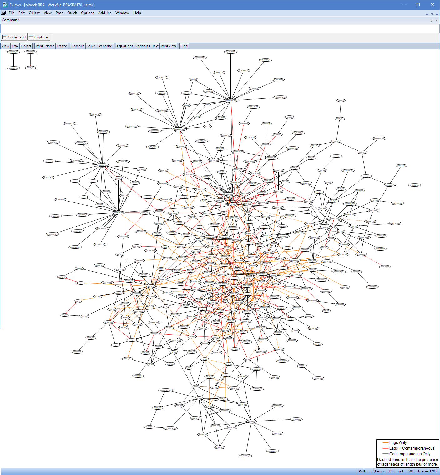
2) Model Dependency Graph

We’ve developed a new way to graphically view the relationship between variables in your model. Colour coding is used to depict the dynamics in the model, and you can zoom and highlight variables for even greater clarity.

Many central banks and large corporations around the world use EViews to build macroeconomic models, and the EViews model object is at the heart of the modelling experience inside EViews.
Whilst EViews has always provided a powerful interface for creating, editing and solving these models. However, it can be difficult for the modeller to explain his work to colleagues and clients. The new dependency graph provides a simple visual guide to how the relationships in the model are structured, allowing demonstration of the structure of the model.


We plan on improving and adding to the dependency graph feature over the next few releases.  If you have any suggestions or requests for the graph (or any other aspect of EViews!) please contact us.

See a complete list of Testing and Diagnostics features added in EViews 10.

3) Bureau of Labor Statistics (BLS) Data

EViews can now connect to the United States Bureau of Labor Statistics’ API to natively fetch data directly from the BLS into EViews.

The US BLS is an important statistical agency, collecting and producing data on labor economics, including vital macroeconomic statistics such as prices (CPI), employment and unemployment, and salary data for both the United States in total, as well as regional aggregates.

The BLS data is also available in other database sources that EViews supports, such as FRED database. However, adding BLS as a direct data source allows for a quicker data retrieval.

See a complete list of Data Handling features added in EViews 10.


4) X-13 Force Option


EViews’ implementation of the U.S. Census Bureau’s X-13 seasonal adjustment package has been extended to give an interface to the Force specification of X-13, which allows you to seasonally adjust the data, forcing the annual totals to remain at the pre-adjusted levels.

Although use of the Force option was possible in previous versions of EViews, EViews 10+ provides a new interface to the option, making its use even easier.

Many economic time series have seasonal cycles; consumption or expenditures increase and decrease at certain times of the year. Most official statistics are seasonally adjusted to remove these cycles to allow analysis of the underlying trends in the data excluding the seasonality.

X-13 has become the de-facto standard method of seasonally adjusting monthly and quarterly time series data within the United States and many other countries, and many agencies use the Force option within X-13 as a method of ensuring the adjusted data lines up with the original raw data. The inclusion of this option to the EViews X-13 interface allows easy access to this popular feature.

See a complete list of Computation features added in EViews 10, including other seasonal adjustment routines.

5) Program Snapshots

EViews 10 introduced the popular workfile snapshot system, allowing both manual and automatic backup, archiving and management of workfiles. EViews 10+ expands this system to EViews program files. You can manually create a snapshot of your EViews program, or let EViews automatically create backups at specified time intervals. Once snapshots have been made you can compare the current version of your program with its snapshots, quickly viewing the differences between the two, and reverting to a previous state if required.


See a complete list of EViews Interface features added in EViews 10.

6) Help Command

A new help command has been implemented which provides a quick way to access the documentation for a specific command.

See a complete list of EViews Interface features added in EViews 10.

State Space Models with Fat-Tailed Errors and the sspacetdist add-in

$
0
0
Author and guest post by Eren Ocakverdi.


Linear State Space Models (LSSM) provide a very useful framework for the analysis of a wide range of time series problems. For instance; linear regression, trend-cycle decomposition, smoothing, ARIMA, can all be handled practically and dynamically within this flexible system.
One of the assumptions behind LSSM is that the errors of the measurement/signal equation are normally distributed. In practice, however, there are situations where this may not be the case and errors follow a fat-tailed distribution. Ignoring this fact may result in wider confidence intervals for the estimated parameters or may cause outliers to bias parameter estimates.

Treatments for heavy-tailed distributions covered in detail in Durbin and Koopman (2012), where they use mode estimates. The following is a signal plus noise model:
$$y_t = \omega_t + \epsilon_t$$
Here, $\omega_t$ is linear Gaussian, and $\epsilon_t$ follows a Student's t-distribution. Observation variance is then given by:
$$A_t = \frac{(v-2)\sigma_\epsilon^2 + \tilde{\epsilon_t^2}}{(v+1)}$$
The Kalman filter and smoother can be applied iteratively to obtain a new smooth estimate of $θ_t$. New values for the signal estimates $\tilde{\epsilon_t}$ are used to compute new values for $A_t$ until convergence to $\epsilon_t$.
This iterative procedure is not built in to EViews, but there is no an add-in, sspacetdist, that allows it. The add-in implements Mean Absolute Percentage Error (MAPE) as the preferred performance metric for convergence.
As an example, Durbin and Koopman (2012) analyze the logged quartely demand for gas in the UK from 1960 to 1986 (gas_data.wf1). They use a structural time series model of the basic form:
$$y_t = \mu_t + \gamma_t + \epsilon_t$$ Here, $\mu_t$ is the local linear trend, $\gamma_t$ is the seasonal component and $\epsilon_t$ is the observation disturbance. We can use the SSpace object of EViews to build this framework and then estimate the model via sspacetdist add-in (sspacet_example1.prg).
The example program file will also generate the Fig. 14.4 on page 318 of Durbin and Koopman (2012). Upper left and right panels are the estimated seasonal components from Gaussian and Student’s t model, respectively. Lower left and right panels are the estimated irregular components of these models, respectively.


Please note that this is an approximating model, but can still be very useful in practice. As another example, let’s simulate a two independent variables regression model with t-distributed errors:
$$y_t = 0.6*x_{1t} + 0.3*x_{2t} + \epsilon_t\text{, where } \epsilon_t \sim t(v=3)$$
Next we estimate the parameters with both maximum likelihood and this iterative state space scheme (sspacet_example2.prg).


Maximum likelihood estimation can be specified within a LogL object. Estimated parameters are close to their theoretical (simulated) values as they all lie within the associated confidence interval.

In order to see how approximating state space model performs, parameters are estimated via add-in:


Note that state space model must be estimated in Gaussian form first. Smoothed state values correspond to coefficients of independent variables and they are very close to the ones estimated by maximum likelihood, which is the true approach for this problem.

As for the degrees-of-freedom parameter, a separate distribution fitting exercise on smoothed disturbances is required. Again, two values are very close (both can be rounded to 3.32).

Note: Interested reader can estimate these models assuming errors are normally distributed and see how confidence intervals of parameters change.


Reference:
Durbin, J. and Koopman, S. J., (2001). Time Series Analysis by State Space Methods, 2nd ed., Oxford University Press.

Using Facebook Likes and Google Trends data to forecast tourism

$
0
0
This post is guest authored by Ulrich Gunter, Irem Önder, Stefan Gindl, all from MODUL University Vienna, and edited by the EViews team.  (Note: all images on this post are for illustrative purposes only; are not taken from the published article and do not represent the exact analysis performed for the article). 

A recent article, "Exploring the predictive ability of LIKES of posts on the Facebook pages of four major city DMOs in Austria" in the scholarly journal Tourism Economics investigates the predictive ability of Facebook “likes” and Google Trends data on tourist arrivals in four major Austrian cities.  The use of online “big data” to perform short term forecasts or nowcasts is becoming increasingly important across all branches of economic study, but is particularly powerful in tourism economics.


A quick graph of Google Trends data for the Austrian city of Salzburg compared with tourist arrivals to the same city shows an obvious correlation:

The article used a number of EViews’ automatic and manual forecasting techniques introduced in recent versions to take advantage of this predictive power.
A brief outline of the steps taken to perform this analysis is as follows:
  • Monthly tourist arrivals for the four cities of Graz, Innsbruck, Salzburg and Vienna are obtained from the TourMIS database.
  • Daily Facebook likes on each city’s official Facebook pages are obtained using Facebook’s Graph API.
  • Monthly Google Trends data for each city is obtained from the Google Trends website.
  • Once data was obtained it is imported into EViews, using different pages for the different frequencies.
  • Seasonal adjustment, unit root tests (with automatic lag-selection) and frequency conversion of daily data to monthly aggregates are all performed in EViews prior to estimation and forecasting.


  • Perform univariate automatic model selection on the arrivals data using automatic ARIMA estimation and automatic ETS smoothing.


  • ADL models regressing tourist arrivals against monthly aggregated Facebook likes or Google Trends, or both, are estimated.  Lag lengths are automatically selected.

  • MIDAS regressions of monthly arrivals against daily Facebook Likes and monthly Google Trends are estimated.
  • Using the EViews programming language, all the above estimation techniques are automated and used to perform recursive forecasts with horizons of 1, 2, 3, 6, 12 and 24 months.
  • Finally, the EViews forecast evaluation tool is used to figure out the best-performing forecast models per city and forecast horizon (in terms of RMSE, MAE, and MAPE). The forecast encompassing test is also utilized.

The results from this analysis are mixed - for two of the cities, the univariate automatic forecasting methods perform best.  For the third city, the ADL model is best, and for the fourth city, the MIDAS approach is best.

Dissecting the business cycle and the BBQ add-in

$
0
0
Authors and guest blog by Davaajargal Luvsannyam and Khuslen Batmunkh

Dating of business cycle is a very crucial for policy makers and businesses. Business cycle is the upward and downward trend of the production or business. Especially macro business cycle, which represents the general economic prospects, plays important role for policy and management decisions. For instance, when the economy is in downtrend companies tend to act more conservative. In contrast, when the economy is in uptrend companies tend to act more aggressive with the purpose of enhancing their market share. Keynesian business cycle theory suggests that business cycle is an important indicator for monetary policy which is able to stabilize the fluctuations of the economy. Therefore accurate dating of business cycle can be fundamental to efficient and practical policy decisions.

In the academic study, the dating process of the business cycle has been changed from a graphical orientation towards quantitative measures extracted from parametric models. For instance, Burns and Mitchell (1946) explained the main concepts of the business cycle and introduced a graphical (classical) model that aims to calculate the peak and trough of the cycle. While Cooley and Prescott (1995) started to calculate the cycle by using the variable moments of the parametric (detrend) models.

Burns and Mitchell define that business cycle is a pattern seen in any series, Yt , taken to represent aggregate economic activity. In the process of defining a cycle, we usually use the logarithm of series Yt . Business cycles are identified as having four distinct phases: trough, expansion, peak, and contraction (Figure 1).

Figure 1. Business Cycle

These are the characteristics of a cycle. Peak (A) is the turning point when the expansion transitions into the contraction phase. Trough (C) is the turning point when the contraction transitions into the expansion phase.  Duration (AB length) is the number of quarters between peak and trough. Amplitude (BC length) is the height of differences between peak and trough.

Figure 2. Illustration of the Contraction Phase

The EViews add-in “BBQ” implements the methodology outlined in Harding and Pagan (2002). Harding and Pagan (2002) chose three countries, the US, the UK and Australia and established turning points for each country by using Bry-Broschan algorithm.  This algorithm performs the following three steps.
  1. Estimation of the possible turning points, i.e. the troughs and peaks in a series.
  2. A technique for alternating the troughs and the peaks.
  3. A set of rules that meet pre-determined criteria of the duration and amplitudes of phases and complete cycles after step 1 and 2.

We will replicate the result of Table 1 of Harding and Pagan (2002).  The example program file (bbq_ex1.prg) will generate  the result.  First we need to open the data file named as hpagan.wf1.

wfopen hpagan.wf1


Data of hpagan.wf1 is quaterly real GDP of the three countries. The sample size for the US is 1947q1 to 1997q1, for the UK 1955q1 to 1997q1 and for Australia 1959q1 to 1997q1.

Next we take the logarithm of series us, uk and aust. 

series lus=log(us)
series luk=log(uk)
series laust=log(aust)

Then we apply the bbq add-in to each series. We can do this either by command line or menu driven interface.

lus.bbq(turnphase=2, phase=2, cycle=5, thresh=10.4)
luk.bbq(turnphase=2, phase=2, cycle=4, thresh=10.4)
laust.bbq(turnphase=2, phase=2, cycle=5, thresh=10.4)


By definition, a peak happens at time t if Yt-k,…,Yt-k+1 < Yt > Yt+1,…,Yt+k  . k needs to be set for example k=2 for quarterly data, k=5 for monthly data and k=1 for yearly data. k is called the symmetric window parameter (turn phase).

Other restrictions are often imposed on the phases. Minimum 2 quarters for expansions and contractions are often applied, in line with the rules used by NBER when dating these phases. This is the minimum phase. A complete cycle length (contraction plus expansion duration) of five quarters is also common for quarterly data. This is the minimum cycle. Finally, it may sometimes be desirable to overrule the minimum phase restriction. For example, if the fall in a series is very large one might allow the contraction to be quite short. The parameter controlling this is threshold (thresh).

Also the add-in produces dummy variables for expansions and contractions (state, state1 and state2)  
Alternatively you can implement the BBQ add-in by menu driven interface. In order to do so first open the series, i.e lus. Then go to proc/add-ins menu and choose Bry-Broschan-Pagan-Harding BC dating menu.


References:
Bry and Boschan (1971). "Cyclical Analysis of Time Series: Selected Procedures and Computer Programs", NBER, New York.
Burns, A., Mitchell, W. C. (1946). "Measuring Business Cycles (Vol. 2)." New York, NY: National Bureau of Economic Research
Cooley and Prescott (1995) ʺEconomic Growth and Business Cyclesʺ Frontiers of Business Cycle Research, ed. Thomas F. Cooley, Princeton University Press, 1‐38.
Pagan and Harding (2002) "Dissecting the cycle: a methodological investigation", Journal of Monetary Economics, Volume 49, Issue 2, 365-381.


Principal Component Analysis Part I (Theory)

$
0
0
Most students of econometrics are taught to appreciate the value of data. We are generally taught that more data is better than less, and that throwing data away is almost "taboo". While this is generally good practice when it concerns the number of observations per variable, it is not always recommended when it concerns the number of variables under consideration. In fact, as the number of variables increases, it becomes increasingly more difficult to rank the importance (impact) of any given variable, and can lead to problems ranging from basic overfitting, to more serious issues such as multicollinearity or model invalidity. In this regard, selecting the smallest number of the most meaningful variables -- otherwise known as dimensionality reduction -- is not a trivial problem, and has become a staple of modern data analytics, and a motivation for many modern techniques. One such technique is Principal Component Analysis (PCA).

Variance Decomposition

Consider a linear statistical system -- a random matrix (multidimensional set of random variables) $ \mathbf{X} $ of size $ n \times m $ where the first dimension denotes observations and the second variables. Moreover, recall that linear statistical systems are characterized by two inefficiencies: 1) noise and 2) redundancy. The former is commonly measured through the signal (desirable information) to noise (undesirable information) ratio $ \text{SNR} = \sigma^{2}_{\text{signal}} / \sigma^{2}_{\text{noise}} $, and implies that systems with larger signal variances $ \sigma^{2}_{\text{signal}} $ relative to their noise counterpart, are more informative. Assuming that noise is a nuisance equally present in observing each of the $ m $ variables of our system, it stands to reason that variables with larger variances have larger SNRs, therefore carry relatively richer signals, and are in this regard relatively more important, or principal. Whereas relative importance reduces to relative variances across system variables, redundancy, or relative uniqueness of information, is captured by system covariances. Recall that covariances (or normalized covariances called correlations) are measures of variable dependency or co-movement (direction and magnitude of joint variability). In other words, variables with overlapping (redundant) information will typically move in the same direction with similar magnitudes, and will therefore have non-zero covariances. Conversely, when variables share little to no overlapping information, they exhibit small to zero linear dependency, although statistical dependence could still manifest nonlinearly. Together, system variances and covariances quantify the amount of information afforded by each variable, and how much of that information is truly unique. In fact, the two are typically derived together using the familiar variance-covariance matrix formula: $$ \mathbf{\Sigma}_{X} = E \left( \mathbf{X}^{\top}\mathbf{X} \right) $$ where $ \mathbf{\Sigma}_{X} $ is an $ m\times m $ square symmetric matrix with (off-)diagonal elements as (co)variances, and where we have a priori assumed that all variables in $ \mathbf{X} $ have been demeaned. Thus, systems where all variables are unique will result in a diagonal $ \mathbf{\Sigma}_{X} $, whereas those exhibiting redundancy will have non-zero off-diagonal elements. In this regard, systems with zero redundancy have a particularly convenient feature known as variance decomposition. Since covariance terms in these systems are zero, total system variation (and therefore information) is the sum of all variance terms, and the proportion of total system information contributed by a variable is the ratio of its variance to total system variation. Although the variance-covariance matrix is typically not diagonal, suppose there exists a way to diagonalize $ \mathbf{\Sigma}_{X} $, and by extension transform $ \mathbf{X} $, while simultaneously preserving information. If such transformation exists, one is guaranteed a new set of at most $ m $ variables (some variables may be perfectly correlated with others) which are uncorrelated, and therefore linearly independent. Accordingly, discarding any one of those new variables would have no linear statistical impact on the $ m-1 $ remaining variables, and would reduce dimensionality at the cost of losing information to the extent contained in the discarded variables. In this regard, if one could also quantify the amount of information captured by each of the new variables, order the latter in descending order of information quantity, one could discard variables from the back until sufficient dimensionality reduction is achieved, while maintaining the maximum amount of information within the preserved variables. We summarize these objectives below:
  1. Diagonalize $ \mathbf{\Sigma}_{X} $.
  2. Preserve information.
  3. Identify principal (important) information.
  4. Reduce dimensionality.
So how does one realize these objectives? It is precisely this question which motivates the subject of this entry.

Principal Component Analysis

Recall that associated with every matrix $ \mathbf{X} $ is a basis -- a set (matrix) of linearly independent vectors such that every row vector in $ \mathbf{X} $ is a linear combination of the vectors in the basis. In other words, the row vectors are projections onto the column vectors in $ \mathbf{B} $. Since the covariance matrix contains all noise and redundancy information associated with a matrix, the idea driving principal component analysis is to re-express the original covariance matrix using a basis that results in a new, diagonal covariance matrix -- in other words, off-diagonal elements in the original covariance matrix are driven to zero and redundancy is eliminated.

Change of Basis

The starting point of PCA is the change of basis relationship. In particular, if $ \mathbf{B} $ is an $ n\times p $ matrix of geometric transformations with $ p \leq m $, the $ n\times p $ matrix $ \mathbf{Q}=\mathbf{XB} $ is a projection of the $ n\times m $ matrix $ \mathbf{X} = [\mathbf{X}_{1}^{\top}, \ldots, \mathbf{X}_{n}^{\top}]^{\top}$ onto $ \mathbf{B} $. In other words, the rows of $ \mathbf{X} $ are linear combinations of the column vectors in $ \mathbf{B} = [\mathbf{B}_{1}, \ldots, \mathbf{B}_{p}]$. Formally, \begin{align*} \mathbf{Q} & = \begin{bmatrix} \mathbf{X}_{1}\\ \vdots\\ \mathbf{X}_{n} \end{bmatrix} \begin{bmatrix} \mathbf{B}_{1} &\cdots &\mathbf{B}_{p} \end{bmatrix}\\ &= \begin{bmatrix} \mathbf{X}_{1}\mathbf{B}_{1} &\cdots &\mathbf{X}_{1}\mathbf{B}_{p}\\ \vdots &\ddots &\vdots\\ \mathbf{X}_{n}\mathbf{B}_{1} &\cdots &\mathbf{X}_{n}\mathbf{B}_{p} \end{bmatrix} \end{align*} More importantly, if the column vectors $ \left\{ \mathbf{B}_{1}, \ldots, \mathbf{B}_{p} \right\} $ are also linearly independent, then $ \mathbf{B} $, by definition, characterizes a matrix of basis vectors for $ \mathbf{X} $. Furthermore, the covariance matrix of this transformation formalizes as: \begin{align} \mathbf{\Sigma}_{Q} = E\left( \mathbf{Q}^{\top}\mathbf{Q} \right) = E\left( \mathbf{B}^{\top}\mathbf{X}^{\top}\mathbf{XB} \right) = \mathbf{B}^{\top}\mathbf{\Sigma}_{X}\mathbf{B} \label{eq1} \end{align} It is important to reflect here on the dimensionality of $ \mathbf{\Sigma}_{Q} $, which, unlike $ \mathbf{\Sigma}_{X} $, is of dimension $ p\times p $ where $ p \leq m $. In other words, the covariance matrix under the transformation $ \mathbf{B} $ is at most the size of the original covariance matrix, and possibly smaller. Since dimensionality reduction is clearly one of our objectives, the transformation above is certainly poised to do so. However, the careful reader may remark here: if the objective is simply dimensionality reduction, then any matrix $ \mathbf{B} $ of size $ n \times p $ with $ p\leq m $ will suffice; so why especially does $ \mathbf{B} $ have to characterize a basis? The answer is simple: dimensionality reduction is not the only objective, but one among preservation of information and importance of information. As to the former, we recall that what makes a set of basis vectors special is that they characterize entirely the space on which an associated matrix takes values and therefore span the multidimensional space on which that matrix resides. Accordingly, if $ \mathbf{B} $ characterizes a basis, then information contained in $ \mathbf{X} $ is never lost during the transformation to $ \mathbf{Q} $. Furthermore, recall that the channel for dimensionality reduction that motivated our discussion earlier was never intended to go through a sparser basis. Rather, the mechanism of interest was a diagonalization of the covariance matrix followed by variable exclusion. Accordingly, any dimension reduction that reflects basis sparsity via $ p \leq m $, is a consequence of perfect co-linearity (correlation) among some of the original system variables. In other words, $ p = \text{rk}\left( \mathbf{X} \right) $, where $ \text{rk}(\cdot) $ denotes the matrix rank, or the number of its linearly independent columns (or rows).

Diagonalization

We argued earlier that any transformation from $ \mathbf{X} $ to $ \mathbf{Q} $ that preserves information must operate through a basis transformation $ \mathbf{B} $. Suppose momentarily that we have in fact found such $ \mathbf{B} $. Our next objective would be to ensure that $ \mathbf{B} $ also produces a diagonal $ \mathbf{\Sigma}_{Q} $. In this regard, we remind the reader of two famous results in linear algebra:
  1. [Thm. 1:] A matrix is symmetric if and only if it is orthogonally diagonalizable.
    • In other words, if a matrix $ \mathbf{A} $ is symmetric, there exists a diagonal matrix $ \mathbf{D} $ and a matrix $ \mathbf{E} $ which diagonalizes $ \mathbf{A} $, such that $ \mathbf{A} = \mathbf{EDE}^{\top} $. The converse statement holds as well.
  2. [Thm. 2:] A symmetric matrix is diagonalized by a matrix of its orthonormal eigenvectors.
    • Extending the result above, if a $ q\times q $ matrix $ \mathbf{A} $ is symmetric, the diagonalizing matrix $ \mathbf{E} = [\mathbf{E}_{1}, \ldots, \mathbf{E}_{q}]$, the diagonal matrix $ \mathbf{D} = \text{diag} [\lambda_{1}, \ldots, \lambda_{q}] $, and $ \mathbf{E}_{i} $ and $ \lambda_{i} $ are respectively the $ i^{\text{th}} $ eigenvector and associated eigenvalue of $ \mathbf{A} $.
    • Note that a set of vectors is orthonormal if each vector is of length unity and orthogonal to all other vectors in the set. Accordingly, if $ \mathbf{V} = [\mathbf{V}_{1}, \ldots, \mathbf{V}_{q}]$ is orthonormal, then $ \mathbf{V}_{j}^{\top}\mathbf{V}_{j} = 1 $ and $ \mathbf{V}_{j}^{\top}\mathbf{V}_{k} = 0 $ for all $ j \neq k $. Furthermore, $ \mathbf{V}^{\top}\mathbf{V} = \mathbf{I}_{q} $ where $ \mathbf{I}_{q} $ is the identity matrix of size $ q $, and therefore, $ \mathbf{V}^{\top} = \mathbf{V}^{-1} $.
    • Recall further that eigenvectors of a linear transformation are those vectors which only change magnitude but not direction when subject to said transformation. Since any matrix is effectively a linear transformation, if $ \mathbf{v} $ is an eigenvector of some matrix $ \mathbf{A} $, it satisfies the relationship $ \mathbf{Av} = \lambda \mathbf{v} $. Here, associated with each eigenvector is the eigenvalue $ \lambda $ quantifying the resulting change in magnitude.
    • Finally, observe that matrix rank determines the maximum number of eigenvectors (eigenvalues) one can extract for said matrix. In particular, if $ \text{rk}(\mathbf{A}) = r \leq q $, there are in fact only $ r $ orthonormal eigenvectors associated with $ \mathbf{A} $. To see this, use a geometric interpretation to note that $ q- $dimensional objects reside in spaces with $ q $ orthogonal directions. Since any $ n\times q $ matrix is effectively a $ q- $dimensional object of vectors, the maximum number of orthogonal directions that characterize these vectors is $ q $. Nevertheless, if the (column) rank of this matrix is in fact $ r \leq q $, then $ q - r $ of the $ q $ orthogonal directions are never used. For instance, think of 2$ d $ drawings in 3$ d $ spaces. It makes no difference whether the drawing is characterized in the $ xy $, the $ xz $, or the $ yz $ plane -- the drawing still has 2 dimensions and in any of those configurations, the dimension left out is a linear combination of the others. In particular, if the $ xz $ plane is used, then the $ z- $direction is a linear combination of the $ y- $direction since the drawing can be equivalently characterized in the $ xy $ plane, and so on. In other words, one of the three dimensions is never used, although it exists and can be characterized if necessary. Along the same lines, if $ \mathbf{A} $ indeed has rank $ r \leq q $, we can construct $ q - r $ additional orthogonal eigenvectors to ensure dimensional equality in the diagonalization $ \mathbf{A} = \mathbf{EDE}^{\top} $, although their associated eigenvalues will in fact be 0, essentially negating their presence.
    • By extension of the previous point, since $ \mathbf{A} $ is a $ q- $dimensional object of $ q- $dimensional column vectors, it can afford at most $ q $ orthogonal directions to characterize its space. Since all $ q $ such vectors are collected in $ \mathbf{E} $, we are guaranteed that $ \mathbf{E} $ is a spanning set and therefore constitutes an eigenbasis.
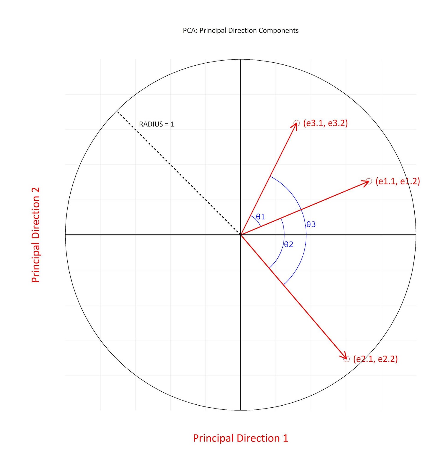
Since $ Cov(\mathbf{X}) $ is a symmetric matrix by construction, the $ 1^{\text{st}} $ result above affords a re-express of equation (\ref{eq1}) as follows: \begin{align} \mathbf{\Sigma}_{Q} &= \mathbf{B}^{\top} \mathbf{\Sigma}_{X} \mathbf{B} \notag \\ &= \mathbf{B}^{\top}\mathbf{E}_{X}\mathbf{D}_{X}\mathbf{E}_{X}^{\top} \mathbf{B} \label{eq2} \end{align} where $ \mathbf{E}_{X} = [\mathbf{E}_{1}, \ldots, \mathbf{E}_{m}] $ is the orthonormal matrix of eigenvectors of $ \mathbf{\Sigma}_{X} $ and $ \mathbf{D}_{X} = \text{diag} [\lambda_{1}, \ldots, \lambda_{q}] $ is the diagonal matrix of associated eigenvalues. Now, since we require $ \mathbf{\Sigma}_{Q} $ to be diagonal, we can set $ \mathbf{B}^{\top} = \mathbf{E}^{-1} $ in order to reduce $ Cov(\mathbf{Q}) $ to the diagonal matrix $ \mathbf{D}_{X} $. Since the $ 2^{\text{nd}} $ linear algebra result above guarantees that $ \mathbf{E}_{X} $ is orthonormal, we know that $ \mathbf{E}^{-1} = \mathbf{E}^{\top} $. Accordingly, \begin{align} \mathbf{\Sigma}_{Q} = \mathbf{D}_{X} \quad \text{if and only if} \quad \mathbf{B} = \mathbf{E}_{X} \label{eq3} \end{align} The entire idea is visualized below in Figures 1 and 2. In particular, Figure 1 demonstrates the ``data perspective'' view of the system in relation to an alternate basis. That is, two alternate basis axes, labeled as ``Principal Direction 1'' and ``Principal Direction 2'' are superimposed on the familiar $ x $ and $ y $ axes. Since the vectors of a basis are mutually orthogonal, the principal direction axes are naturally drawn at $ 90 $&deg angles. Alternatively, Figure 2 demonstrates the view of the system when the perspective uses the principal directions as the reference axes.


Consistency

In practice, $ \mathbf{\Sigma}_{X} $, and by extension $ \mathbf{\Sigma}_{Q}, \mathbf{E}_{X}, $ and $ \mathbf{D}_{X} $, are typically not observed. Nevertheless, we can apply the analysis above using sample covariance matrices $$ \mathbf{S}_{Q} = \frac{1}{n}\mathbf{Q}^{\top}\mathbf{Q} \xrightarrow[n \to \infty]{p} \mathbf{\Sigma}_{Q} \quad \text{and} \quad \mathbf{S}_{X} = \frac{1}{n}\mathbf{X}^{\top}\mathbf{X} \xrightarrow[n \to \infty]{p} \mathbf{\Sigma}_{X} $$ where $ \xrightarrow[\color{white}{n \to \infty}]{p} $ indicates weak convergence to asymptotic counterparts. In this regard, the result analogous to equation (\ref{eq2}) for estimated $ 2^{\text{nd}} $ moment matrices states that \begin{align} \mathbf{S}_{Q} = \widehat{\mathbf{E}}_{X}^{\top} \mathbf{S}_{X} \widehat{\mathbf{E}}_{X} = \widehat{\mathbf{E}}_{X}^{\top} \left( \widehat{\mathbf{E}}_{X}\widehat{\mathbf{D}}_{X}\widehat{\mathbf{E}}_{X}^{\top} \right) \widehat{\mathbf{E}}_{X} = \widehat{\mathbf{D}}_{X} \label{eq4} \end{align} where $ \widehat{\mathbf{E}}_{X} $ and $ \widehat{\mathbf{D}}_{X} $ now represent the eigenbasis and respective eigenvalues associated with the square symmetric matrix $ \mathbf{S}_{X} $. It is important to understand here that while $ \widehat{\mathbf{E}}_{X} \neq \mathbf{E}_{X} $ and $ \widehat{\mathbf{D}}_{X} \neq \mathbf{D}_{X} $, there is a long-standing literature far beyond the scope of this entry which guarantees that $ \widehat{\mathbf{E}}_{X} $ and $ \widehat{\mathbf{D}}_{X} $ are both consistent estimators of $ \mathbf{E}_{X} $ and $ \mathbf{D}_{X} $, provided $ m/n \to 0 $ as $ n \to \infty $. In other words, as in classical regression paradigms, consistency of PCA holds only under the usual ``large $ n $ and small $ m $ '' framework. There are modern results which address cases for $ m/n \to c > 0 $, however, they too are beyond the scope of this text. In proceeding however, in order to contain notational complexity, unless otherwise stated, we will maintain that $ \mathbf{E}_{X} $ and $ \mathbf{D}_{X} $ now represent the eigenbasis and respective eigenvalues associated with the square symmetric matrix $ \mathbf{S}_{X} $.

Preservation of Information

In addition to diagonalizing $ \mathbf{S}_{Q} $, we also require preservation of information. For this we need to guarantee that $ \mathbf{B} $ is a basis. Here, we recall the final remark under the $ 2^{\text{nd}} $ linear algebra result above, which argues that $ \mathbf{S_{Q}} $ affords at most $ m $ orthonormal eigenvectors and associated eigenvalues, with the former also forming an eigenbasis. Since all $ m $ eigenvectors are collected in $ \mathbf{E}_{X} = \mathbf{B} $, we are guaranteed that $ \mathbf{B} $ is indeed a basis. In this regard, we transform $ \mathbf{X} $ into $ m $ statistically uncorrelated, but exhaustive directions. We are careful not to use the word variables (although technically they are), since the transformation $ \mathbf{Q} = \mathbf{XE}_{X} $ does not preserve variable interpretation. That is, the $ j^{\text{th}} $ column of $ \mathbf{Q} $ no longer retains the interpretation of the $ j^{\text{th}} $ variable (column) in $ \mathbf{X} $. In fact, the $ j^{\text{th}} $ column of $ \mathbf{Q} $ is a projection (linear combination) of all $ m $ variables in $ \mathbf{X} $, in the direction of the $ j^{\text{th}} $ eigenvector $ \mathbf{E}_{j} $. Accordingly, we can interpret $ \mathbf{XE}_{X} $ as $ m $ orthogonal weighted averages of the $ m $ variables in $ \mathbf{X} $. Furthermore, since $ \mathbf{E}_{X} $ is an eigenbasis, the total variation (information) of the original system $ \mathbf{X} $, namely $ \mathbf{S}_{X} $, is preserved in the transformation to $ \mathbf{Q} $. Unlike $ \mathbf{S}_{X} $ however, $ \mathbf{S}_{Q} = \mathbf{D}_{X}$ is diagonal, and total variation in $ \mathbf{X} $ is now distributed across $ \mathbf{Q} $ without redundancy.

Principal Directions

Since preservation of information is guaranteed under the transformation $ \mathbf{Q} = \mathbf{XE}_{X} $, the proportion of information in $ \mathbf{S}_{X} $ associated with the $ j^{\text{th}} $ column of $ \mathbf{S}_{Q}$ is in fact $ \lambda_{j} $. By extension, each column in $ \mathbf{Q} $ has standard deviation $ \sqrt{\lambda_{j}} $ or variance $ \lambda_{j} $. Moreover, since $ \mathbf{S}_{Q} $ is diagonal and information redundancy is not an issue, it stands to reason that the total amount of system variation is the sum of variations due to each column in $ \mathbf{Q} $. In other words, total system variation is $ \text{tr}\left( \mathbf{S}_{Q} \right) = \lambda_{1} + \ldots + \lambda_{m} $, where $ \text{tr}(\cdot) $ denotes the matrix trace operator, and the $ j^{\text{th}} $ orthogonalized direction contributes to $$ \frac{\lambda_{j}}{\lambda_{1} + \ldots + \lambda_{m}} \times 100 \% $$ of total system variation (information). If we now arrange the columns of $ \mathbf{Q} $, or equivalently those of $ \mathbf{E}_{X} $, according to the order $ \lambda_{(1)} \geq \lambda_{(2)} \geq \ldots \geq \lambda_{(m)} $, where $ \lambda_{(j)} $ are ordered versions of their counterparts $ \lambda_{j} $, we are guaranteed to have the directions arranged from most principal to least, measured as the proportion of total system variation contributed by that direction. Another useful feature of the vectors in $ \mathbf{E}_{X} $ is that they quantify the proportion of directionality each original variable contributes toward the overall direction of that vector. In particular, let $ e_{i,j} $ denote the $ i^{\text{th}} $ element in $ \mathbf{E}_{j} = [e_{1,j}, \ldots, e_{m,j} ]$, where $ i \in {1, \ldots, m} $, and observe that since $ \mathbf{E}_{j} $ are the eigenvectors of $ \mathbf{S}_{X} $, each element $ e_{i,j} $ is in fact associated with the $ i^{\text{th}} $ variable (column) of $ \mathbf{X} $. Furthermore, since the vectors $ \mathbf{E}_{j} $ each have unit length due to (ortho)normality, we know that they must lie inside the unit circle and that $ e_{i,j}^{2} \times 100 \% $ of the direction $ \mathbf{E}_{j} $ is due to variable $ i $. In other words, we can quantify how principal each variable is in each direction.

Principal Components

Principal directions, the eigenvectors in $ \mathbf{E}_{X} $, are often mistakenly called principal components. Nevertheless, correct literature reserves the term principal components for the projections of the original system variables onto the principal directions. That is, principal components refer to the column vectors in $ \mathbf{Q} = [\mathbf{Q}_{1}, \ldots, \mathbf{Q}_{m}] = \mathbf{XE}_{X} $, and are sometimes also referred to as scores. Like their principal direction counterparts, principal components contain several important properties worth observing. As a direct consequence of the diagonalization properties discussed earlier, the variance of each principal component is in fact the eigenvalue associated with the underlying principal direction, and principal components are mutually uncorrelated. To see this formally, let $ \mathbf{C}_{j} = [0, \ldots, 0, \underbrace{1}_j, 0, \ldots, 0 ]^{\top} $ denote the canonical basis vector in the $ j^{\text{th}} $ dimension. Then, using the result in equation (\ref{eq4}), the correlation between the $ j^{\text{th}} $ and $ k^{\text{th}} $ principal components $ \mathbf{Q}_{j} = \mathbf{QC}_{j} $ and $ \mathbf{Q}_{k} = \mathbf{QC}_{k} $, respectively, is obviously: \begin{align*} s_{Q_{j}, Q_{k}} &= \frac{1}{n}\mathbf{Q}_{j}^{\top}\mathbf{Q}_{k} \\ &= \mathbf{C}_{j}^{\top} \left( \frac{1}{n} \mathbf{Q}^{\top}\mathbf{Q} \right) \mathbf{C}_{k} \\ &= \mathbf{C}_{j}^{\top} \mathbf{S}_{Q} \mathbf{C}_{k} \\ &= \mathbf{C}_{j}^{\top} \mathbf{D}_{X} \mathbf{C}_{k} \\ \end{align*} which equals $ \lambda_{j} $ when $ j = k $ and $ 0 $ otherwise. Moreover, we can quantify how (co)related the original variables are with the principal directions. In particular, consider the covariance between the $ i^{\text{th}} $ variable $ \mathbf{X}_{i}=\mathbf{XC}_{i} $ and the $ j^{\text{th}} $ principal component $ \mathbf{Q}_{j} $, formalized as: \begin{align} \mathbf{S}_{X_{i}Q_{j}} & = \frac{1}{n} \mathbf{X}_{i}^{\top}\mathbf{Q}_{j} \notag\\ &= \mathbf{C}_{i}^{\top} \left( \frac{1}{n}\mathbf{X}^{\top}\mathbf{Q} \right) \mathbf{C}_{j}\notag\\ &= \mathbf{C}_{i}^{\top} \left( \frac{1}{n}\mathbf{X}^{\top}\mathbf{X}\mathbf{E}_{X} \right) \mathbf{C}_{j}\notag\\ &= \mathbf{C}_{i}^{\top} \mathbf{S}_{X} \mathbf{E}_{X} \mathbf{C}_{j}\notag\\ &= \mathbf{C}_{i}^{\top} \mathbf{E}_{X}\mathbf{D}_{X} \mathbf{E}_{X}^{\top} \mathbf{E}_{X} \mathbf{C}_{j}\notag\\ &= \mathbf{C}_{i}^{\top} \mathbf{E}_{X}\mathbf{D}_{X} \mathbf{C}_{j}\notag\\ &= e_{i,j} \lambda_{j} \label{eq5} \end{align} where the antepenultimate line invokes Theorem 1 to $ \mathbf{S}_{X} $, and the cancelation to identity in the penultimate line follows by Theorem 2 and orthonormality of $ \mathbf{E}_{X} $, and the ultimate line is the product of the $ j^{\text{th}} $ element of the principal direction $ \mathbf{E}_{j} $ and the $ j^{\text{th}} $ principal eigenvalue.

Dimension Reduction

At last, we arrive a the issue of dimensionality reduction. Assuming that the columns of $ \mathbf{Q} $ are arranged in decreasing order of importance (more principal columns come first), we can discard the $ g < m $ least principal columns of $ \mathbf{Q} $ until sufficient dimension reduction is achieved, and rest assured that the remaining (first) $ m - g $ columns are in fact most principal. In other words, the $ m - g $ directions which are retained, contribute to $$ \frac{ \sum \limits_{j=1}^{m-g}\lambda_{(j)}}{\lambda_{1} + \ldots + \lambda_{m}} \times 100 \% $$ of the original variation in $ \mathbf{X} $. Since directions are ordered in decreasing order of importance, the first few directions will capture the majority of variation, leaving the less principal directions to contribute information only marginally. Accordingly, one can significantly reduce dimensionality whilst retaining the majority of information. This is particularly important when we want to measure the complexity of our data set. In particular, if the $ r $ most principal directions account for the majority of variance, it stands to reason that our underlying data set is in fact only $ r- $dimensional, with the remaining $ m-r $ dimensions being noise. In other words, dimensionality reduction naturally leads to data denoising. So how does one select how many principal directions to retain? There are several approaches, but we list only several below:
  1. A very popular approach is to use a scree plot -- a plot of the ordered eigenvalues from most to least principal. The idea here is to look for a sharp drop in the function, and select the bend or elbow as the cutoff value, retaining all eigenvalues (and by extension principal directions) to the left of this value.
  2. Another popular alternative is to use the cumulative proportion of variation explained by the first $ r $ principal directions. In other words, select the first $ r $ principal directions such that $ \frac{ \sum \limits_{j=1}^{r}\lambda_{(j)}}{\lambda_{1} + \ldots + \lambda_{m}} \geq 1 - \alpha $, where $ \alpha \in [0,1] $. Typical uses set $ \alpha = 0.1 $ in order to retain $ r $ most principal directions that capture at least 90\% of the system variation.
  3. A more data driven result is known as the Guttman-Kaiser (Guttman (1954), Kaiser (1960), Kaiser (1961)) criterion. This criterion advocates the retention of all eigenvalues, and by extension, the associated principal directions, that exceed the average of all eigenvalues. In other words, select the first $ r $ principal directions such that $ \lambda_{(1)} + \ldots + \lambda_{(k)} \geq r\bar{\lambda} $, where $ \bar{\lambda} = \frac{1}{m} \sum\limits_{j = 1}^{m}\lambda_{j} $.
  4. An entirely data-driven approach akin to classical information criteria selection methods borrows the Bai and Ng (2002) paper on factor models. In this regard, consider $$ \mathbf{X}_{j} = \beta_{1}\mathbf{Q}_{1} + \ldots + \beta_{k}\mathbf{Q}_{r} + \mathbf{U}(j,r) $$ as the regression of the $ j^{\text{th}} $ variable in $ \mathbf{X} $ on the first $ k $ principal directions of $ \mathbf{S}_{X} $, and let $ \widehat{\mathbf{U}}(j,r) $ denote the corresponding residual vector. Furthermore, define $ SSR(j,r) = \frac{1}{n} \widehat{\mathbf{U}}(j,r)^{\top} \widehat{\mathbf{U}}(j,r) $ as the sum of squared residuals from said regression, and define $ SSR(r) = \frac{1}{m}\sum \limits_{j=1}^{m}SSR(j,r) $ as the average of all $ SSR(j,r) $ across all variables $ j $ for a given $ r $. We can then select $ r $ as the one that minimizes a particular penalty function. In other words, the problem reduces to: $$ \min\limits_{r} \left\{ \ln\left( SSR(k) \right) + rg(n,m) \right\} $$ where $ g(n,m) $ is a penalty term which leads to one of several criteria proposed in Bai and Ng (2002). For instance when $ n > m $, one such option is the $ IC_{p2}(r) $ criterion, and the problem above formalizes as: $$ \min\limits_{r} \left\{ \ln\left( SSR(r) \right) + r\left( \frac{n + m}{nm} \right) \ln(m) \right\} $$
Of course, it goes without saying that discarding information comes at its own cost, although, if dimensionality reduction is desired, it may well be a price worth paying.

Inference

Although PCA is deeply rooted in linear algebra, it is also a very visual experience. In this regard, a particularly convenient feature is the ability to visualize multidimensional structures across two-dimensional summaries. In particular, comparing two principal directions provides a wealth of information that is typically inaccessible in traditional multidimensional contexts.

Loading Plots

A powerful inferential tool unique to PCA is element-wise comparison of two principal directions. In particular, consider two principal directions $ \mathbf{E}_{j} = [e_{1,j}, \ldots, e_{m,j}]$ and $ \mathbf{E}_{k} = [e_{1,k}, \ldots, e_{m,k}]$, and let $ \left\{ \mathbf{V}_{1,j,k}, \ldots, \mathbf{V}_{m,j,k} \right\}$ denote the set of vectors from the origin $ (0,0) $ to $ \left( e_{i,j}, e_{i,k} \right) $ for $ i \in {1, \ldots, m} $. In other words, $ \mathbf{V}_{i,j,k} = \left( e_{i,j}, e_{i,k} \right)^{\top}$. Then, for any $ (j,k) $ principal direction pairs, a plot of all $ m $ vectors $ \mathbf{V}_{i,j,k} $, for $ i \in {1, \ldots, m} $, on a single plot, is called a loading plot. There is an important connection between the vectors $ \mathbf{V}_{i,j,k} $ and original variable covariances. In particular, consider $ \mathbf{S}_{X_{i},X_{s}} $ -- the finite sample covariance between $ \mathbf{X}_{i} $ and $ \mathbf{X}_{s} $ -- and, assuming we have ordered eigenvalues from most principal to least, note that: \begin{align*} \mathbf{S}_{X_{i},X_{j}} &= \mathbf{C}_{i}^{\top} \mathbf{S}_{X} \mathbf{C}_{s}\\ &= \mathbf{C}_{i}^{\top} \mathbf{E}_{X} \mathbf{D}_{X} \mathbf{E}_{X}^{\top} \mathbf{C}_{s}\\ &= \lambda_{(1)}e_{i,1}e_{s,1} + \lambda_{(2)}e_{i,2}e_{s,2} + \ldots + \lambda_{(m)}e_{i,m}e_{s,m}\\ &= \mathbf{V}_{i,1,2}^{\top}\mathbf{L}_{1,2}\mathbf{V}_{s,1,2} + \ldots + \mathbf{V}_{i,m-1,m}^{\top}\mathbf{L}_{m,m-1}\mathbf{V}_{s,m-1,m} \end{align*} where $ \mathbf{L}_{j,k} = \text{diag} \left[\lambda_{(j)}, \lambda_{(k)} \right] $ denotes the appropriate scaling matrix. In other words, for any $ (j,k) $ principal direction pairs, $ \mathbf{V}_{i,j,k}^{\top} \mathbf{L}_{j,k} \mathbf{V}_{s,j,k} $ explains a proportion of the covariance $ \mathbf{S}_{X_{i},X_{s}} $. Accordingly, when $ \mathbf{X}_{i} $ and $ \mathbf{X}_{s} $ are highly correlated, we can expect $ \mathbf{V}_{i,j,k}^{\top} \mathbf{L}_{j,k} \mathbf{V}_{s,j,k} $ to be larger values. In this regard, let $ \theta_{i,s,j,k} $ denote the angle between any two vectors $ \mathbf{V}_{i,j,k} $ and $ \mathbf{V}_{s,j,k} $, and recall that \begin{align*} \cos \theta_{i,s,j,k} &= \frac{\mathbf{V}_{i,j,k}^{\top}\mathbf{V}_{s,j,k}}{\norm{\mathbf{V}_{i,j,k}} \norm{\mathbf{V}_{s,j,k}}} \end{align*} To accommodate the use of the scaling matrices $ \mathbf{L}_{j,k} $, observe that we can modify this result as follows: \begin{align} \mathbf{V}_{i,j,k}^{\top} \mathbf{L}_{j,k} \mathbf{V}_{s,j,k} = \mathbf{V}_{i,j,k}^{\top} \mathbf{L}_{j,k} \left(\mathbf{V}_{i,j,k}\mathbf{V}_{i,j,k}^{\top} \right)^{-1} \mathbf{V}_{i,j,k} \norm{\mathbf{V}_{i,j,k}} \norm{\mathbf{V}_{s,j,k}} \cos \theta_{i,s,j,k} \label{eq6} \end{align} Now, when $ \theta_{i,s,j,k} $ is small, say between $ 0 $ and $ \pi/2 $, we can expect $ \mathbf{V}_{i,j,k}^{\top} \mathbf{L}_{j,k} \mathbf{V}_{s,j,k} $ to be large, and by extension, $ \mathbf{X}_{i} $ and $ \mathbf{X}_{s} $ to be more correlated. In other words, vectors that are close to one another in a loading plot indicate stronger correlations of their underlying variables. Figure 3 below gives a visual representation.


It is important to realize here that since $ \theta_{i,s,j,k} $ is in fact the angle between $ \mathbf{V}_{i,j,k} $ and $ \mathbf{V}_{s,j,k} $, the interpretation of how exhibitive $ \theta_{i,s,j,k} $ is of the underlying correlation $ \mathbf{S}_{X_{i}, X_{s}} $ is made more complicated by the presence of $ \mathbf{L}_{j,k} $ in equation (\ref{eq6}). Accordingly, to ease interpretation, the vectors $ \mathbf{V}_{i,j,k} $ are sometimes scaled appropriately, or loaded with scaling information, leading to the term loadings. In this regard, consider the vectors $ \widetilde{\mathbf{V}}_{i,j,k} = \mathbf{V}_{i,j,k} \mathbf{L}_{j,k}^{1/2} $. Here, loading is done via $ \mathbf{L}_{j,k}^{1/2} $, and we have: $$ \mathbf{S}_{X_{i}, X_{s}} = \widetilde{\mathbf{V}}_{i,1,2}^{\top}\widetilde{\mathbf{V}}_{s,1,2} + \ldots + \widetilde{\mathbf{V}}_{i,m-1,m}^{\top}\widetilde{\mathbf{V}}_{s,m-1,m} $$ and $$ \widetilde{\mathbf{V}}_{i,j,k}^{\top}\widetilde{\mathbf{V}}_{s,j,k} = \norm{\widetilde{\mathbf{V}}_{i,j,k}} \norm{\widetilde{\mathbf{V}}_{s,j,k}} \cos \widetilde{\theta}_{i,s,j,k} $$ As such, $ \widetilde{\theta}_{i,s,j,k} $ more closely exhibits the true angle between $ \mathbf{X}_{i} $ and $ \mathbf{X}_{s} $ than $ \theta_{i,s,j,k} $, and loading plots using $ \widetilde{\mathbf{V}}_{i,j,k} $ tend to be more exhibitive of the underlying correlations $ \mathbf{S}_{X_{i}, X_{s}} $ than those based on $ \mathbf{V}_{i,j,k} $. Of course, one does not have to resort to the use of $ \mathbf{L}_{j,k}^{1/2} $ as the loading matrix. In principle, one can use $ \mathbf{L}_{j,k}^{\alpha} $ for some $ \alpha $, although the underlying interpretation of what such a loading means ought to be understood first. Figure 4 below demonstrates the impact of using a loading weight. In particular, the vectors in Figure 3 are superimposed on the set of loaded vectors where the loading factor is $ \mathbf{D}_{X}^{1/2} $. Clearly, the loaded vectors are much more correlated with the general shape of the data as represented by the ellipse.


Scores Plots

A score plot across principal direction pairs $ (j,k) $ is essentially a scatter plot of the principal component vector $ \mathbf{Q}_{i} $ vs. $ \mathbf{Q}_{j} $. In fact, it is the analogous version of the loading plot, but for observations as opposed to variables. In this regard, whereas the angle between two loading vectors is exhibitive of the underlying correlation between some variables, the distance between observations in a score plot exhibits homogeneity across observations. Accordingly, observations which tend to cluster together, tend to move together, and one typically looks to identify important clusters when conducting inference.

Outlier Detection

An important application of PCA is to outlier detection. The general principle exploits the first few principal directions to explain the majority of variation in the original system, and uses data reconstruction to generate an approximation of the original system using the first few principal components. Formally, if we start from the matrix of all principal components $ \mathbf{Q} $, it is trivial to reconstruct the original system $ \mathbf{X} $ using the inverse: $$ \mathbf{Q}\mathbf{E}_{X}^{\top} = \mathbf{X}\mathbf{E}_{X}\mathbf{E}_{X}^{\top} = \mathbf{X}$$ On the other hand, if we restrict our principal components to the first $ r \ll m $ most principal directions, then $ \widetilde{\mathbf{Q}}\widetilde{\mathbf{E}}_{X}^{\top} = \widetilde{\mathbf{X}} \approx \mathbf{X} $, where $ \widetilde{\mathbf{Q}} $ and $ \widetilde{\mathbf{E}}_{X} $ are respectively the matrix $ \mathbf{Q} $ and $ \mathbf{E}_{X} $ with the last $ m - r $ columns removed, and $ \approx $ denotes an approximation. Then, the difference $$ \mathbf{\xi} = \widetilde{\mathbf{X}} - \mathbf{X} $$ is known as the reconstruction error, and if the first $ r $ principal directions explain the original variation well, we can expect $ \norm{\mathbf{\xi}}_{D}^{2} \approx \mathbf{0}$ where $ \norm{\cdot}_{D} $ denotes some measure of distance. We would now like to define a statistic associated with outlier identification, and as in usual regression analysis, the reconstruction error (residuals) plays a key role. In particular, we follow the contributions of Jackson and Mudholkar (1979) and define $$ \mathbf{SPE} = \mathbf{\xi} \mathbf{\xi}^{\top} $$ as the squared prediction error most resembling the usual sum of squared residuals. Moreover, Jackson and Mudholkar (1979) show that if observations (row vectors) in $ \mathbf{X} $ are independent and identically distributed, Gaussian random variables, $ \mathbf{SPE} $ has the following distribution $$ \mathbf{SPE} \sim \sum\limits_{j+1}^{m}\lambda_{(j)}Z_{j}^{2} \equiv \Psi(k) $$ where $ \chi^{2}_{p} $ denotes the $ \chi^{2}- $distribution with $ p $ degrees of freedom, and $ Z_{j} $ are independent $ \chi^{2}_{1} $ variables. Noting that the $ i^{\text{th}} $ diagonal element of $ \mathbf{SPE} $, namely $ \mathbf{SPE}_{ii} = \mathbf{C}_{i}^{\top} \mathbf{SPE} \mathbf{C}_{i} $ is associated with the $ i^{\text{th}} $ observation, we can now derive a rule for outlier detection. In particular, should $ \mathbf{SPE}_{ii} $, for any $ i $, fall into some critical region defined by the upper $ (1 - \alpha) $ percentile of $ \Psi(k) $, that observation would be considered an outlier.

Closing Remarks

Principal component analysis is an extremely important multivariate statistical technique that is often misunderstood and abused. The hope is that in reading this entry you will have found the intuition one often seeks in complicated subject matters, with just enough mathematical rigour to ease any serious future undertakings. In Part II of this series, we will use EViews to exhibit a PCA case study and demonstrate just how easy this is with a a few clicks.

References

[1] Jushan Bai and Serena Ng. Determining the number of factors in approximate factor models. Econometrica, 70(1):191--221, 2002.
[2] Louis Guttman. Some necessary conditions for common-factor analysis. Psychometrika, 19(2):149--161, 1954.
[3] J Edward Jackson and Govind S Mudholkar. Control procedures for residuals associated with principal component analysis. Technometrics, 21(3):341--349, 1979.
[4] Henry F Kaiser. The application of electronic computers to factor analysis. Educational and psychological measurement, 20(1):141--151, 1960.
[5] Henry F Kaiser. A note on guttman's lower bound for the number of common factors 1. British Journal of Statistical Psychology, 14(1):1--2, 1961.

Principal Component Analysis: Part II (Practice)

$
0
0
In Part I of our series on Principal Component Analysis (PCA), we covered a theoretical overview of fundamental concepts and disucssed several inferential procedures. Here, we aim to complement our theoretical exposition with a step-by-step practical implementation using EViews. In particular, we are motivated by a desire to apply PCA to some dataset in order to identify its most important features and draw any inferential conclusions that may exist. We will proceed in the following steps:
  1. Summarize and describe the dataset under consideration.
  2. Extract all principal (important) directions (features).
  3. Quantify how much variation (information) is explained by each principal direction.
  4. Determine how much variation each variable contributes in each principal direction.
  5. Reduce data dimensionality.
  6. Identify which variables are correlated and which correlations are more principal.
  7. Identify which observations are correlated with which variables.
The links to the workfile and program file can be found at the end.

Principal Component Analysis of US Crime Data

We will use PCA to study US crime data. In particular, our dataset summarizes the number of arrests per 100,000 residents in each of the 50 US states in 1973. The data contains four variables, three of which pertain to arrests associated with (and naturally named) MURDER, ASSAULT, and RAPE, whereas the last, named URBANPOP, contains the percentage of the population living in urban centers.

Data Summary

To understand our data, we will first create a group object with the variables of interest. We can do this by selecting all four variables in the workfile by clicking on each while holding down the Ctrl button, right-clicking on any of the highlighted variables, moving the mouse pointer over Open in the context menu, and finally clicking on as Group. This will open a group object in a spreadsheet with the four variables placed in columns. The steps are reproduced in Figures 1a and 1b.


Figure 1A: Open Group

Figure 1B: Group Window

From here, we can derive the usual summary statistics by clicking on View in the group window, moving the mouse over Descriptive Stats and clicking on Common Sample. This produces a spreadsheet with various statistics of interest. We reproduce the steps and output in Figures 2a and 2b.


Figure 2A: Descriptive Stats Menu

Figure 2B: Descriptive Stats Output

We can also plot each of the series to get a better visual sense for the data. In particular, from the group window, click on View and click on Graph. This brings up the Graph Options window. Here, from the Multiple Series dropdown menu, select Multiple Graphs and click on OK. We summarize the sequence in Figures 3a and 3b.


Figure 3A: Graph Options

Figure 3B: Multiple Graphs

At last, we can get a sense for information redundancy (see section Variance Decomposition in Part I of this series) by studying correlation patterns. In this regard, we can produce a correlation matrix by clicking on View in the group window and clicking on Covariance Analysis.... This opens a window with further options. Here, deselect (click) the checkbox next to Covariance and select (click) the box next to Correlation. This ensures that EViews will only produce the correlation matrix without any other statistics. Furthermore, in the Layout dropbox, select Single table, and finally click on OK. Figures 4a and 4b reproduce these steps.


Figure 4A: Covariance Analysis

Figure 4B: Correlation Table

A quick interpretation of the correlation structure indicates that murder is highly correlated with assault, whereas the latter exhibits a strong positive correlation with rape. Moreover, whereas murder is nearly uncorrelated with larger urban centers, among the three causes for arrest, rape generally favours larger communities. Intuitively, this is in line with conventional wisdom. Murders are rarely observed on professional levels and typically involve assault as a precursor. Furthermore, due to higher costs of crime visibility and cleanup, murder generally does not favour larger population areas where police presence and witness visibility is generally more pronounced. On the other hand, rape favours larger urban centers due to the fact that there are simply more people and the cost to covering or denying the crime is notoriously very low. Furthermore, victims of rape in smaller communities are typically shamed into staying quiet since connection circles are naturally tighter in such surroundings.

Principal Component Analysis of Crime Data

Doing PCA in EViews is trivial. From our group object window, click on View and click on Principal Components.... This opens the main PCA dialog. See Figure 5a and 5b below.


Figure 5A: Initiating the PCA dialog

Figure 5B: Main PCA Dialog

From here, EViews offers users the ability to apply several tools and protocols readily encountered in the literature on PCA.

Summary of Fundamentals

As a first step, we are interested in summarizing PCA fundamentals. In particular, we seek an overview of eigenvalues and eigenvectors that result from applying the principal component decomposition to the covariance or correlation matrix associated with our variables of interest. To do so, consider the Display group, and select Table. The latter produces three tables summarizing the covariance (correlation) matrix, and the associated eigenvectors and eigenvalues. Associated to this output are several important options under the Component selection group. These include:
  • Maximum number: This defaults to the theoretical maximum number of eigenvalues possible, which is the total number of variables in the group under consideration. In our case, this number is 4.
  • Minimum eigenvalue: This defaults to 0. Nevertheless, selecting a positive value requests that all eigenvectors associated with eigenvalues less than this value are not displayed.
  • Cumulative proportion: This defaults to 1. Choosing a value $\alpha < 1$ however, requests that only the most principal $ k $ eigenvalues and eigenvectors associated with explaining $ \alpha*100 \% $ of the variation are retained. Naturally, choosing $ \alpha=1 $ requests that all eigenvalues are displayed. See section Dimension Reduction in Part I of this series for further details.
Since we are interested in a global summary, we will leave the Component selection options at their default values. Furthermore, consider momentarily the Calculation tab. Here, the Type dropdown offers the choice to apply the principal component decomposition either to the correlation or covariance matrix. For details, see sections Variance Decomposition and Change of Basis in Part I of this series. The choice essentially reduces to whether or not the variables under consideration exhibit similar scales. In other words, if variances of the underlying variables of interest are similar, then conducting PCA on the covariance matrix is certainly justified. Nevertheless, if the variances are widely different, then selecting the correlation matrix is more appropriate if interpretability and comparability are desired. EViews errs on the side of caution and defaults to using the correlation matrix. Since the table of summary statistics we produced in figure 3b clearly shows a lack of uniformity in standard deviations across the four variables of interest, we will stick with the default and use the correlation matrix. Hit OK.


Figure 6: PCA Table Output

The resulting output, which is summarized Figure 6 above, consists of three tables. The first table summarizes the information on eigenvalues. The latter are sorted in order of principality (importance), measured as the proportion of information explained by each principal direction. Refer to section Principal Directions in Part I of this series for more details. In particular, we see that the first principal direction explains roughly 62% of the information contained in the underlying correlation matrix, the second, roughly 25%, and so on. Furthermore, the cumulative proportion of information explained by the first two principal directions is roughly 87(62 + 25)%. In other words, if dimensionality reduction is desired, our analysis indicates that we can half the underlying dimensionality of the problem from 4 to 2, while retaining nearly 90% of the original information. This is evidently a profitable trade-off. For theoretical details, see section Dimension Reduction in Part I of this series. At last, observe that EViews reports that the average of the 4 eigenvalues is 1. This will in fact always be the case when extracting eigenvalues from a correlation matrix. The second (middle) table summarizes the eigenvectors associated with each of the principal eigenvalues. Naturally, the eigenvectors are also arranged in order of principality. Furthermore, whereas the eigenvalues highlight how much of the overall information is extracted in each principal direction, the eigenvectors reveal how much weight each variable has in each direction. Recall from Part I of this series that all eigenvectors have length unity. Accordingly, the relative importance of any variable in a given principal direction is effectively the proportion of the eigenvector length (unity) attributed to that variable. For instance, in the case of the first eigenvector, $ [0.535899, 0.583184, 0.543432, 0.278191]^{\top} $, MURDER accounts for $ 0.535899^{2} \times 100\% = 0.287188\% $ of the overall direction length. Similarly, ASSAULT accounts for 0.340103% of the direction, and RAPE contributes 0.295318%. Evidently, the least important variable in the first principal direction is URBANPOP, which accounts for only 0.077390% of the direction length. On the other hand, in the second principal direction, it is URBANPOP that carries most weight, contributing $ 0.872806 \times 100\% = 0.761790\% $ to the direction length. Accordingly, if feature extraction is the goal, it is clear (and rather obvious) that the first principal direction is roughly equally dominated by MURDER, ASSAULT, and RAPE, whereas the second principal direction is almost entirely governed by URBANPOP. For a theoretical exposition, see section Principal Components in Part I of this series. At last, the third table is just the correlation matrix to which the eigen-decomposition is applied. The latter, while important, is provided only as a reference.

Eigenvalue Plots and Dimensionality

Now that we have a rough picture of PCA fundamentals associated with our dataset, it is natural to ask whether we can proceed with dimensionality reduction in a more formal manner. One such way (albeit arbitrary, but widely popular) is to look at several eigenvalue plots and visually identify how many eigenvalues to retain. From the previous PCA output, click again on View, then Principal Components..., and select Eigenvalue Plots under the Display group. This is summarized in Figure 7 below.


Figure 7: PCA Dialog: Eigenvalue Plots

Here, EViews offers several graphical representations for the underlying eigenvalues. The latter includes the scree plot, the differences between successive eigenvalues plot, as well as the cumulative proportion of information associated with the first $ k $ eigenvalues plot. Go ahead and select all three. As before, we will leave the default values under the Component Selection group. Hit OK. Figure 8 summarizes the output.


Figure 8: Eigenvalue Plots Output

EViews now produces three graphs. The first is the scree plot - a line graph of eigenvalues arranged in order of principality. Superimposed on this graph is a red dotted horizontal line with a value equal to the average of the eigenvalues, which, as we mentioned earlier, in our case is 1. The idea here is to look for a kink point, or an elbow, and retain all eigenvalues, and by extension their associated eigenvectors, that form the first portion of the kink, and discard the rest. From the plot, it is evident that a kink occurs at the 2nd eigenvalue, indicating that we should retain the first two eigenvalues. A slightly more numeric approach discards all eigenvalues significantly below the eigenvalue average. Referring to the first table in Figure 6, we see that the average of the eigenvalues is 1, and the 2nd eigenvalue is in fact just below this cutoff. Since the 2nd value is so close to this average, while using the visual support we mentioned in the previous paragraph, it is safe to conclude that the scree plot analysis indicates that only the first two eigenvalues ought to be retained. The second graph plots a line graph of the differences between successive eigenvalues. Superimposed on this graph is another horizontal line, this time with a value equal to the average of the differences of successive eigenvalues. Although EViews does not report this number, using the top table in Figure 6, it is not difficult to show that the average in question is $ (1.490476+0.633202+0.183133)/3 = 0.768937 $. The idea here is to retain all eigenvalues whose differences are above this threshold. Clearly, only the first two eigenvalues satisfy this criterion. The final graph is a line graph of the cumulative proportion of information explained by successive principal eigenvalues. Superimposed on this graph is a line with a slope equal to the average of the eigenvalues, namely 1. The idea here is to retain those eigenvalues that form segments of the cumulative curve whose slopes are at least as steep as the line with slope 1. In our case, only two eigenvalues seem to form such a segment: eigenvalues 1 and 2. All three graphical approaches indicate that one ought to retain the first two eigenvalues and their associated eigenvectors. There is however an entirely data driven methodology adapted from Bai and Ng (2002). We discussed this approach in section Dimension Reduction in Part I of this series. Nevertheless, EViews currently doesn't support its implementation via dialogs and it must be programmed manually. In this regard, we temporarily move away from our dialog-based exposition, and offer a code snippet which implements the aforementioned protocol.

' --- Bai and Ng (2002) Protocol ---
group crime murder assault rape urbanpop ' create group with all 4 variables
!obz = murder.@obs ' get number of observations
!numvar = @columns(crime) ' get number of variables
equation eqjr ' equation object to hold regression
matrix(!numvar, !numvar) SSRjr' matrix to store SSR from each regression eqjr

crime.makepcomp(cov=corr) s1 s2 s3 s4 ' get all score series

for !j = 1 to !numvar
for !r = 1 to !numvar
%scrstr = ""' holds score specification to extract

' generate string to specify which scores to use in regression
for !r2 = 1 to !r
%scrstr = %scrstr + " s" + @str(!r2)
next

eqjr.ls crime(!j) {%scrstr} ' estimate regression

SSRjr(!j, !r) = (eqjr.@ssr)/!obz ' take average of SSR
next
next
' get column means of SSRjr. namely, get r means, averaging across regressions j.
vector SSRr = @cmean(SSRjr)

vector(!numvar) IC ' stores critical values
for !r = 1 to !numvar
IC(!r) = @log(SSRr(!r)) + !r*(!obz + !numvar)/(!obz*!numvar)*@log(!numvar)
next

' take the index of the minimum value of IC as number of principal components to retain
scalar numpc = @imin(IC)
Unlike our graphical analysis, the protocol above suggests that the number of retained eigenvalues is 1. Nevertheless, for sake of greater analytical exposition below, we will stick with the original suggestion of retaining the first two principal directions instead.

Principal Direction Analysis

The next step in our analysis is to look at what, if any, meaningful patterns emerge by studying the principal directions themselves. To do so, we again bring up the main principal component dialog and this time select Variable Loading Plots under the Display group. See Figure 9 below.


Figure 9: PCA Dialog: Variable Loading Plots

Variable loading plots produce ``$ XY $ ''-pair plots of loading vectors. See section Loading Plots in Part I of this series for further details. The user specifies which loading vectors to compare and selects one among the following loading (scaling) protocols:
  • Normalize Loadings: In this case, scaling is unity and loading vectors are in fact the eigenvectors themselves.
  • Normalize Scores: Here, the scaling factor is the square root of the eigenvalue vector. In other words, the $ k^{\text{th}} $ element of the $ i^{\text{th}} $ loading vector is the $ k^{\text{th}} $ element of the $ i^{\text{th}} $ eigenvector, multiplied by the square root of the $ k^{\text{th}} $ eigenvalue.
  • Symmetric Weights: In this scenario, the scaling factor is the quartic (fourth) root of the eigenvalue vector. Namely, the $ k^{\text{th}} $ element of the $ i^{\text{th}} $ loading vector is the $ k^{\text{th}} $ element of the $ i^{\text{th}} $ eigenvector, multiplied by the fourth root of the $ k^{\text{th}} $ eigenvalue.
  • User Loading Weight: If $ 0 \leq \omega \leq 1 $ denotes the user defined scaling factor, then the loading vectors are formed by scaling the $ k^{\text{th}} $ element of the corresponding eigenvector by the $ k^{\text{th}} $ eigenvalue raised to the power $ \omega/2 $ .
For the time being, stick with all default values. That is, we will look at the loading plots across the first two principal directions, and we will use the Normalize Loadings scaling protocol. In other words, we will plot the true eigenvectors since scaling is unity. Note that the choice of looking at only the first two principal directions is, among other things, motivated by our previous analysis on dimension reduction where we decided to retain only the first two principal eigenvalues and discard the rest. Go ahead and click on OK. Figure 10 summarizes the output.


Figure 10: Variable Loading Plots Output

As discussed in section Loading Plots in Part I of this series, the angle between the vectors in a loading plot is related to the correlation between the original variables to which the loading vectors are associated. Accordingly, we see that MURDER and ASSAULT are moderately positively correlated, as are ASSAULT and RAPE, although the latter two less so than the former two. Moreover, it is clear that RAPE and URBANPOP are positively correlated, whereas MURDER and URBANPOP are nearly uncorrelated since they form a near 90 degree angle. In other words, we have a two-dimensional graphical representation of the four-dimensional correlation matrix in Figure 4b. This ability to represent higher dimensional information in a lower dimensional space is arguably the most useful feature of PCA. Furthermore, all three variables, MURDER, ASSAULT, and RAPE, are strongly correlated with the first principal direction, whereas URBANPOP is strongly correlated with the second principal direction. In fact, looking at vector lengths, we can also see that MURDER, ASSAULT, and RAPE are roughly equally dominant in the first direction, whereas URBANPOP is significantly more dominant than either of the former three, albeit in the second direction. Of course, this simply confirms our preliminary analysis of the middle table in Figure 6. Above, we started with the basic loading vector with scale unity. We could have, of course, resorted to other scaling options such as normalizing to the score vectors, using symmetric weights, or using some other custom weighting. Since each of these would yield a different but similar perspective, we won't delve further into details. Nevertheless, as an exercise in exhibiting the steps involved, we provide below small snippets of code to manually generate loading vectors using only the eigenvalues and eigenvectors associated with the underlying correlation matrix. This is done for each of the four scaling protocols. These manually generated vectors are then compared to the loading vectors generated by EViews' internal code and shown to be identical.

' --- Verify Loading Plot Vectors ---
group crime murder assault rape urbanpop ' create group with all 4 variables

' make eigenvalues and eigenvectors based on the corr. matrix
crime.pcomp(eigval=eval, eigvec=evec, cov=corr)

'normalize loadings
crime.makepcomp(loading=load, cov=corr) s1 s2 s3 s4 ' EViews generated loading vectors
matrix evaldiag = @makediagonal(eval) ' create diagonal matrix of eigenvalues
matrix loadverify = evec*evaldiag ' manually create loading vector with scaling unity
matrix loaddiff = loadverify - load ' get difference between custom and eviews output
show loaddiff ' display results

'normalize scores
crime.makepcomp(scale=normscores, loading=load, cov=corr) s1 s2 s3 s4
loadverify = evec*@epow(evaldiag, 0.5)
loaddiff = loadverify - load
show loaddiff

'symmetric weights
crime.makepcomp(scale=symmetrics, loading=load, cov=corr) s1 s2 s3 s4
loadverify = evec*@epow(evaldiag, 0.25)
loaddiff = loadverify - load
show loaddiff

'user weights
crime.makepcomp(scale=0.36, loading=load, cov=corr) s1 s2 s3 s4
loadverify = evec*@epow(evaldiag, 0.18)
loaddiff = loadverify - load
show loaddiff

Score Analysis

Whereas loading vectors reveal information on which variables dominate (and by how much) each principal direction, it is only when they are used to create the principal component vectors (score vectors) that they are truly useful in a data exploratory sense. In this regard, we again open the main principal component dialog and select Component scores plots in the Display group of options. We capture this in Figure 11 below.


Figure 11: PCA Dialog: Component Scores Plots

Analogous to the loading vector plots, here, EViews produces ``$ XY $ ''-pair plots of score vectors. As in the case of loading plots, the user specifies which score vectors to compare, and selects one among the following loading (scaling) protocols:
  • Normalize Loadings: Score vectors are scaled by unity. In other words, no scaling occurs.
  • Normalize Scores: The $ k^{\text{th}} $ score vector is scaled by the inverse of the square root of the $ k^{\text{th}} $ eigenvalue.
  • Symmetric Weights: The $ k^{\text{th}} $ score vector is scaled by the inverse of the quartic root of the $ k^{\text{th}} $ eigenvalue.
  • User Loading Weight: If $ 0 \leq \omega \leq 1 $ denotes the user defined scaling factor, the $ k^{\text{th}} $ score vector is scaled by the $ k^{\text{th}} $ eigenvalue raised to the power $ -\omega/2 $.
Furthermore, if outlier detection is desired, EViews allows users to specify a p-value as a detection threshold. See sections Score Plots and Outlier Detection in Part I of this series for further details. Since we are currently interested in interpretive exercises, we will forgo outlier detection and choose to display all observations. To do so, under the Graph options group of options, change the Obs. Labels to Label all obs. and hit OK. We replicate the output in Figure 12.


Figure 12: Component Scores Plots Output

The output produced is a scatter plot of principal component 1 (score vector 1) vs. principal component 2 (score vector 2). There are several important observations to be made here. First, the further east of the zero vertical axis a state is located, the more positively correlated it is with the first principal direction. Since the latter is dominated positively (east of the zero vertical axis) by the three crime categories MURDER, ASSAULT, and RAPE (see Figure 11), we conclude that such states are positively correlated with said crimes. Naturally, converse conclusions hold as well. In particular, we see that CALIFORNIA, NEVADA, and FLORIDA are most positively correlated with the three crimes under consideration. If this is indeed the case, then it is little surprise that most Hollywood productions typically involve crime thrillers set in these three states. Conversely, NORTH DAKOTA and VERMONT are typically least associated with the crimes under consideration. Second, the further north of the zero horizontal axis a state is located, the more positively correlated it is with the second principal direction. Since the latter is dominated positively (north of the zero horizontal axis) by the variable URBNAPOP (see Figure 11), we conclude that such states are positively correlated with urbanization. Again, the converse conclusions hold as well. In particular, HAWAII, CALIFORNIA, RHODE ISLAND, MASSACHUSETTS, UTAH, NEW JERSEY are states most positively associated with urbanization, whereas those least so are SOURTH CAROLINA, NORTH CAROLINA, and MISSISSIPPI. Lastly, it is worth recalling that like loading vectors, score vectors can also be scaled. In this regard, we provide code snippets below to show how to manually compute scaled score vectors, exposing the algorithm that EViews uses to do same in its internal computations.

' --- Verify Score Vectors ---
' make eigenvalues and eigenvectors based on the corr. matrix
crime.pcomp(eigval=eval, eigvec=evec, cov=corr)

matrix evaldiag = @makediagonal(eval) ' create diagonal matrix of eigenvalues

stom(crime, crimemat) ' create matrix from crime group
vector means = @cmean(crimemat) ' get column means
vector popsds = @cstdevp(crimemat) ' get population standard deviations

' initialize matrix for normalized crimemat
matrix(@rows(crimemat), @columns(crimemat)) crimematnorm

' normalize (remove mean and divide by pop. s.d.) every column of crimemat
for !k = 1 to @columns(crimemat)
colplace(crimematnorm,(@columnextract(crimemat,!k) - means(!k))/popsds(!k),!k)
next

'normalize loadings
crime.makepcomp(cov=corr) s1 s2 s3 s4 ' get score series
group scores s1 s2 s3 s4 ' put scores into group
stom(scores, scoremat) ' put scores group into matrix
matrix scoreverify = crimematnorm*evec ' create custom score matrix
matrix scorediff = scoreverify - scoremat ' get difference between custom and eviews output
show scorediff

'normalize scores
crime.makepcomp(scale=normscores, cov=corr) s1 s2 s3 s4
group scores s1 s2 s3 s4
stom(scores, scoremat)
scoreverify = crimematnorm*evec*@inverse(@epow(evaldiag, 0.5))
scorediff = scoreverify - scoremat
show scorediff

'symmetric weights
crime.makepcomp(scale=symmetrics, cov=corr) s1 s2 s3 s4
group scores s1 s2 s3 s4
stom(scores, scoremat)
scoreverify = crimematnorm*evec*@inverse(@epow(evaldiag, 0.25))
scorediff = scoreverify - scoremat
show scorediff

'user weights
crime.makepcomp(scale=0.36, cov=corr) s1 s2 s3 s4
group scores s1 s2 s3 s4
stom(scores, scoremat)
scoreverify = crimematnorm*evec*@inverse(@epow(evaldiag, 0.18))
scorediff = scoreverify - scoremat
show scorediff
Above, observe that we derived eigenvalues and eigenvectors of the correlation matrix. Accordingly, to derive the score vectors manually, we needed to standardize the original variables first. In this regard, when using the covariance matrix instead, one need only to demean the original variables and disregard scaling information. We leave this as an exercise to interested readers.

Biplot Analysis

As a last exercise, we superimpose the loading vectors and score vectors onto a single graph called the biplot. To do this, again, bring up the main principal component dialog and under the Display group select Biplot (scores & loadings). As in the previous exercise, under the Graph options group, select Label all obs. from the Obs. labels dropdwon, and hit OK. We summarize these steps in Figure 13.


Figure 13: PCA Dialog: Biplots (scores & loadings)

From an inferential standpoint, there's little to contribute beyond what we laid out in each of the previous two sections. Nevertheless, having both the loading and score vectors appear on the same graph visually reinforces our previous analysis. Accordingly, we close this section with just the graphical output.


Figure 14: Biplots (scores & loadings) Output

Concluding Remarks

In Part I of this series we laid out the theoretical foundations underlying PCA. Here, we used EViews to conduct a brief data exploratory implementation of PCA on serious crimes across 50 US states. Our aim was to illustrate the use of numerous PCA tools available in EViews with brief interpretations associated with each. In closing, we would like to point out that apart from the main principal component dialog we used above, EViews also offers a Make Principal Components... proc function which provides a unified framework for producing vectors and matrices of the most important objects related to PCA. These include the vector of eigenvalues, the matrix of eigenvectors, the matrix of loading vectors, as well as the matrix of scores. To access this function, open the crime group from the workfile, click on Proc and click on Make Principal Components.... We summarize this in Figures 15a and 15b below.


Figure 15a: Group Proc: Make Principal Components...

Figure 15b: Make Principal Components Dialog

From here, one can insert names for all objects one wishes to place in the workfile, select the scaling one wishes to use in the creation of the loading and score vectors, and hit OK.

Files

The EViews workfile can be downloaded here: usarrests.wf1 The EViews program file can be downloaded here: usarrests.prg

References

[1] Jushan Bai and Serena Ng. Determining the number of factors in approximate factor models. Econometrica, 70(1):191--221, 2002.

Nowcasting GDP on a Daily Basis

$
0
0
Author and guest blog by Michael Anthonisz, Queensland Treasury Corporation.
In this blog post, Michael demonstrates the use of MIDAS in EViews to nowcast Australian GDP growth on a daily basis.

"Nowcasts" are forecasts of the here and now ("now" + "forecast" = "nowcast"). They are forecasts of the present, the near future or the recent past. Specifically, nowcasts allow for real-time tracking or forecasting of a lower frequency variable based on other series which are released at a similar or higher frequency.


For example, one could try to forecast the outcome for the current quarter GDP release using a combination of daily, weekly, monthly and quarterly data. In this example, the nowcast could be updated on a daily basis – the highest frequency of explanatory data – as new releases for the series being used to explain GDP came in. That is, as the daily, weekly, monthly and quarterly data used to explain GDP is released, the nowcast for current quarter GDP is updated in real-time on a daily basis.

The ability to update one's forecast incrementally in real-time in response to incoming information is an attractive feature of nowcasting models. Forecasting in this manner will lower the likelihood of one's forecasts becoming "stale". Indeed, nowcasts have been found to be more accurate:

  • at short-term horizons.
  • as the period of interest (eg, the current quarter) goes on.
  • than traditional forecasting approaches at these horizons.
Other key findings in relation to nowcasts are that:
  • they also perform similarly to private sector forecasters who are able to also incorporate information in real-time.
  • there are mixed findings as to relative gains from including high frequency financial data.
  • "soft data"1 is most useful early on in the nowcasting cycle and "hard data"2 is of more use later on.
There are a number of approaches that can be used to prepare a nowcast including:

Through its broad functionality EViews is able to facilitate the use of all of these approaches. For the purposes of this blog entry and in recognition of its availability from EViews 9.5 onwards as well as its ease of use, MIDAS regressions will be used to provide a daily nowcast of quarterly trend Australian real GDP growth5. MIDAS models are perfectly suited to handle the nowcasting problem, which at its essence, relates to how to use data for explanatory variables which are released at different frequencies to explain the dependent variable6.

In this example, the series used in the MIDAS model to nowcast GDP are not just regular economic or financial time series, however. To capture as broad a variety of influences on the dependent variable as possible, as well as to ensure a parsimonious specification, principal components analysis ("PCA") is used7. This allows us to extract a common trend from a large number of series. Using this approach will enable us to cut down on "noise" and hopefully use more "signal" to estimate GDP.

The data series used to derive these common factors are compiled on a monthly and quarterly basis and are released in advance of, during and following the completion of the current quarter of interest with respect to GDP. The common factors are calculated at the lowest frequency of the underlying data (quarterly) and are complemented in the model by daily financial data which may have some explanatory power over the quarterly change in Australian GDP (for example, the trade weighted exchange rate and the three-year sovereign bond yield).

An outline of the steps required to do this sort of MIDAS-based nowcast is below. Keep in mind the helpful point and click as well as command language instructions published by EViews which provide more detail.
  • Create separate tabs in the workfie which correspond to the different frequencies of underlying data you are using.
  • Import the underlying data and normalize to be in Z Score form (that is, mean of zero and variance of one) before running the PCA.
  • Have the common factors created from the PCA appear on the relevant tab in the workfile8.
  • Clean the data to get rid of any N/A values for data that has not yet been published.9
  • Re-run the PCA to reflect that you now have data for the underlying series for the full sample period.
It is important to note that the variable being nowcast must actually be forecast with the same periodicity as its release. In this instance, GDP is released quarterly so our forecasts of it will be quarterly as well. This means all the work at this stage of the estimation will be done on the quarterly page. We are aiming
to produce forecasts of a quarterly variable which are updated on a more real-time (that is, daily basis) but are not actually producing a forecast of daily GDP.

An illustration of the rolling process might make this clearer. For instance:
  • Let's imagine it is currently 1 July 2018.
  • We’re interested in forecasting Q3 2018 GDP using one period lags of GDP and the common factors estimated earlier via PCA. These are quarterly representations of conditions with respect to labour markets and capital investment as well as measures of current and future economic activity. We’ll also using bond yields and the trade-weighted exchange rate, both of which are available on a daily basis.
  • In our MIDAS model, quarterly GDP is the dependent variable and the aforementioned other variables are independent variables. The model is estimated using historical data from Q2 1993 until Q2 2018 (as it is 1 July we have data to 30 June).
  • As we want to forecast Q3, and have data on our daily variables until the end of Q2 2018, we can specify the equation as each quarter’s GDP growth is a function of the previous quarter’s outcomes for the quarterly variable and of (say) the last 45 days’ worth of values for bond yields and the exchange rate ending on the last day of the previous quarter.
  • Having estimated the model, we can use the 45 daily values for bond yields and the exchange rate from May to June 2018 to forecast Q3 GDP.
  • Now, assume the calendar has turned over and it is now 2 July 2018. We have one more observation for the daily series. We can update the forecast of GDP by estimating a new model on historical data that used 44 days from the previous quarter and the first day from the current quarter, and then forecast Q3 GDP.
  • Then, assume it is 3 July 2018. We can now update our forecast by estimating on 43 days of the previous quarter and the first 2 days from the current quarter. And so on.
  • We will end up with a forecast of quarterly GDP that is updated daily. That doesn't make it a forecast of daily GDP as it is a quarterly variable. We're just able to forecast it using current (now) data and update this forecast continuously on a daily basis.
For our concrete example using Australian macroeconomic variables, we will estimate a MIDAS model where the dependent variable is the quarterly change in the trend measure of Australian real GDP.

The independent variables of the model can be seen in Figure 1:
Figure 1: Independent variables used in MIDAS estimation (click to enlarge)
All data are sourced from the Bloomberg and Thomson Reuters Datastream databases, accessible via EViews.

The specific equation in EViews is estimated using the Equation object with the method set to MIDAS, and with variable names of:
  • gdp_q_trend_3m_chg = quarterly change in the trend measure of Australian GDP.
  • gdp_q_trend_3m_chg(-1) = one quarter lag of the quarterly change in the trend measure of Australian GDP.
  • activity_current(-1) = one quarter lag of a PCA derived factor representing current economic activity in Australia.
  • activity_leading(-1) = one quarter lag of a PCA derived factor representing future economic activity in Australia.
  • investment(-1) = one quarter lag of a PCA derived factor representing capital investment in Australia.
  • labour_market(-1) = one quarter lag of a PCA derived factor representing labour market conditions in Australia.
  • au_midas_daily\atwi_final(-1) = the lag of the trade-weighted Australia Dollar where this data is located on a page with a daily frequency.
  • au_midas_daily\gacgb3_final(-1) = the lag of the three-year Australian sovereign bond yield where this data is located on a page with a daily frequency.
In this example we will estimate the dependent variable using historical data from Q2 1993 until Q2 2018. From this we can then do forecasts for the current quarter (in this case Q3 2018) whereby the dependent variable is a function of the previous quarter’s outcomes for the quarterly independent variables and of the last 45 days’ worth of values for bond yields and the exchange rate. The MIDAS equation estimation window that reflects this would be as follows:
Figure 2: Estimation specification (click to enlarge)

Running the MIDAS model results in the following estimation output:
Figure 3: Estimation output (click to enlarge)
This individual estimation gives us a single forecast for GDP based upon the most current data available. Specifically, this estimation uses data up to:
  • 2018Q2 for our dependent variable.
  • 2018Q1 for our quarterly independent variables (since they are all lagged one period).
  • May 30th for our daily independent variables (a one day lag from the last day of Q2). Also note that since we are using 45 daily periods for each quarter, the 2018Q2 data point is estimated using data from March 29th - May 30th (we are dealing with regular 5-day data).
From this equation we can then produce a forecast of the 2018Q3 value of GDP by clicking on the Forecast button:
Figure 4: Forecast dialog (click to enlarge)
This single quarter forecast uses data from:
  • 2018Q2 for our quarterly independent variables (since they are all lagged one period).
  • July 30th 2018 - September 28th 2018 for our daily independent variables (45 days ending on the last day of Q3 2018 - September 29th/30th are a weekend, so not included in our workfile).
To produce an updated forecast the following day, we could re-estimate our equation using the same data, but with the daily independent variables shifted forwards one day (removing the one day lag on their specification), and then re-forecasting.

Or, if we wanted an historical view on how our forecasts would have performed previously, we can re-estimate for the previous day (shifting our daily variables back by one day by increasing their lag to 2) and then re-forecast.

Indeed we could repeat the historical procedure going back each day for a number of years, giving us a series of daily updated forecast values. Performing this action manually is a little cumbersome, but an EViews program can make the task simple. A rough example of such a program may be downloaded here.

Once the series of daily forecasts is created, you can produce a good picture of the accuracy of this procedure:
Figure 5: Daily updated forecast of Australian GDP Trend (click to expand)


1 Such as consumer or business surveys
2 Such a retail spending, housing or labour market data
3 As GDP, for example, is essentially an accounting identity that represents the sum of different income, expenditure or production measures, it can be calculated using a ‘bottom-up’ approach in which series that proxy for the various components of GDP are used to construct an estimate of it using an accounting type approach.
4 Bridge equations are regressions which relate low frequency variables (e.g. quarterly GDP) to higher frequency variables (eg, the unemployment rate) where the higher frequency observations are aggregated to the quarterly frequency. It is often the case that some but not all of the higher frequency variables are available at the end of the quarter of interest. Therefore, the monthly variables which aren’t as yet available are forecasted using auxiliary models (eg, ARIMA).
5 Papers using a daily frequency in mixed frequency regression analyses include Andreou, Ghsels & Kourtellos, 2010, Tay, 2006 and Sheen, Truck & Wang, 2015.
6 MIDAS models use distributed lags of explanatory variables which are sampled at an equivalent or higher frequency to the dependent variable. A distributed lag polynomial is used to ensure a parsimonious specification. There are different types of lag polynomial structures available in EViews. Lindgren & Nilson, 2015 discuss the forecasting performance of the different polynomial lag structures.
7 See here and here for background and here and here for how to do in EViews.
8 For example, underlying data on a monthly and quarterly basis will generate a common factor that is on a quarterly basis. This should therefore go on a quarterly workfile tab.
9 For example, if there was an NA then you could choose to use the previous value for the latest date instead. For example, X_full series = @recode(X =na, X(-1), X)

Panel Structural VARs and the PSVAR add-in

$
0
0
Author and guest blog by Davaajargal Luvsannyam

Panel SVARs have been used to address a variety of issues of interest to policymakers and applied economists. Panel SVARs are particularly suitable to analyze the transmission of idiosyncratic shocks across units and time. For example, Canova et al. (2012) have studied how U.S. interest rate shocks are propagated to 10 European economies, 7 in the Euro area and 3 outside of it, and how German shocks are transmitted to the remaining nine economies. 


Panel SVARs have also been often used to estimate average effects – possibly across heterogeneous groups of units - and to describe unit specific differences relative to the average. For example, researcher may analyze if monetary policy is more countercyclical, on average, in countries or states.  Researcher may also be interested in knowing whether inflation dynamics in states may depend on political, geographical, cultural or institutional features, or on whether monetary and fiscal interactions are related. 

Alternative potential use of panel SVARs is in studying the importance of interdependencies, and in checking whether reactions are generalized or only involve certain pairs of units. Therefore, some researchers want to implement a panel SVARs to evaluate certain exogeneity assumptions or to test the small open economy assumption, often made in the international economics literature.


In this blog, we describe the econometric estimation and implementation of the Panel SVAR of Pedroni (2013). The key to Pedroni (2013) estimation and identification method will be the assumption that structural shocks can be decomposed into both common and idiosyncratic structural shocks, which are mutually orthogonal.


Structural shock representation

Associated with the $M\times1$ vector of demeaned panel data, $z_{it}$, let $\xi_{it} = \left(\bar{\epsilon}_t^\prime, \tilde{\epsilon}_{it}^\prime\right)^\prime$ where $\bar{\epsilon}_t^\prime$ and $\tilde{\epsilon}_{it}^\prime$ are $M\times 1$ vectors of common and idiosyncratic white noise shocks, respectively. Let $\Lambda_i$ be and $M\times M$ diagonal matrix such that the diagonal elements are the loading coefficients $\lambda_{i,m}$, where $m=1,\ldots, M$. Then the composite white noise errors, \begin{equation} \epsilon_{it} = \Lambda_i \bar{\epsilon}_t + \tilde{\epsilon}_{it} \end{equation} where $E\left[ \xi_{it}\xi_{it}^\prime \right] = \text{diag} \left\{ \Omega_{i, \bar{\epsilon}}, \Omega_{i, \tilde{\epsilon}} \right\}, \forall i,t$. Moreover, $E\left[\xi_{it}\right] = 0, \forall i,t$, $E\left[\xi_{is}\xi_{it}^\prime\right] = 0, \forall i,s\neq t$, and $E\left[\tilde{\epsilon}_{it}\tilde{\epsilon}_{it}^\prime\right] = 0, \forall i\neq j, t$.

Relationships between reduced forms and structural forms

\begin{align*} &\text{Shocks:} \quad \mu_{it} = A_i(0)\epsilon_{it}\\ &\text{Responses:} \quad F_{i}(L)A_i(0) = A_i(L)\\ &\text{Steady states:} \quad F_{i}(1)A_i(0) = A_i(1) \end{align*} where $\mu_{it}$ is the reduced form residuals ($R_i(L) \Delta z_{it} = \mu_{it}$), $F_i(L) = R_i(L)^{-1}$, and $\epsilon_{it}$ are the structural shocks ($\delta z_{it} = A_i(L)\epsilon_{it}$).

Typical structural identifying restrictions on dynamics

\begin{align*} &A(0) \text{ decompositions:} \quad \Omega_{\mu,i} = A_i(0)A_i(0)^\prime\\ &\text{Short-run restrictions:} \quad \Omega_{\mu,i} = B_i(0)^{-1}B_i(0)^{-1^\prime}\\ &\text{Long-run restrictions:} \quad \Omega_{\mu,i}(1) = A_i(1)A_i(1)^\prime \end{align*} The adding-up of constraints with re-normalization implies that equation (1) can be rewritten as $$\epsilon_{it} = \Lambda_i \bar{\epsilon}_{it} + (I - \Lambda_i\Lambda_i^\prime)^{1/2} \tilde{\epsilon}_{it}^\star$$ Finally, we can use this re-scaled form to decompose the impulse responses into the common and idiosyncratic shocks as: $$ A_i(L) = \bar{A}_i(L) + \tilde{A}_i(L)$$ where $\bar{A}_i(L)$ is the member specific response to the common shocks ($\bar{A}_i(L) = A_i(L)\Lambda_i$), and $\tilde{A}_i(L)$ is the member specific response to the idiosyncratic shocks ($\tilde{A}_i(L) = A_i(L)(I - \Lambda_i\Lambda_i^\prime)^{1/2}$) such that the two responses sum to the total member specific response to the composite shocks. The following is a summary of the estimation algorithm for an unbalanced panel $\Delta z_{i,t}$ with dimensions $i = 1, \ldots, N$(member), $t=1, \ldots T_i$(time), and $m=1, \ldots, M)$(variable):
  1. Compute the time effects, $\Delta \bar{z}_t = N_t^{-1}\sum_{i=1}^{N_t}\Delta z_{it}$ and use these along with $\Delta z_{it}$ to estimate the reduced form VARs, $\bar{R}(L)\Delta \bar{z}_t = \bar{mu}_t$ and $R_i(L)\Delta z_{it} = \mu_{it}$ for each member $i$, using an information criterion to fit an appropriate member specific lag truncation, $P_i$.
  2. Use appropriate identifying restrictions such as short-run (Cholesky) or long-run (BQ) identification method to obtain structural shock estimates for $\epsilon_{it}$(composite) and $\bar{\epsilon}_{t}$(common).
  3. Compute diagonal elements of the loading matrix, $\Lambda_i$, as correlations between $\epsilon_{it}$ and $\bar{\epsilon}_t$ for each member, $i$, and compute idiosyncratic shock, $\tilde{\epsilon}_{it}$, using equation $\epsilon_{it} = \Lambda_i \bar{\epsilon}_t + \tilde{\epsilon}_{it}$.
  4. Compute member-specific impulse responses to unit shocks: $A_i(L) = \bar{A}_i(L) + \tilde{A}_i(L)$, where $\bar{A}_i(L) = A_i(L)\Lambda_i$ and $\tilde{A}_i(L) = A_i(L)(I - \Lambda_i\Lambda_i^\prime)^{1/2}$
  5. Use sample distribution of estimated $A_i(L), \bar{A}_i(L)$, and $\tilde{A}_i(L)$ responses to describe properties of the confidence interval quantiles.

Now we turn to the implementation of the psvar add-in. First, we need to open the data file named as pedroni_ppp.wf1 which is located in the installation folder. 
wfopen pedroni_ppp.wf1

For testing purpose, we use this panel data. The sample size for the data is 4920 (1973m06 to 1993m11 x 20)  

Next, we generate variable, ereal, and take the logarithm of series ereal, cpi and ae. You don’t need take the first difference of variables. The add-in will do it for you. 

series ereal = ae*uscpi/cpi
series logereal = log(Ereal)   
series logcpi = log(cpi)     
series logae = log(ae)

Then we apply the psvar add-in to this panel data. We can do this either by command line or menu driven interface. 

psvar(ident=2, horizon=24) 18 @ logereal logcpi logae

or

psvar(ident=2, horizon=24, ci=0.5, length=5, average=mean, sample=”1976m06 1993 m11”, save=1) 18 @ logereal logcpi logae

Please see the document for the detailed description of the command options. The resulting output will be three graph objects that contains 3x3 charts similar to those produced by EViews’ VAR object: 
Figure 1: Response Estimates to Composite Shocks

Figure 2: Response Estimates to Common Shocks

Figure 3: Response Estimates to Idiosyncratic Shocks
Alternatively, you can implement the psvar add-in by the menu driven interface.


The first box lets you specify the endogenous variable (logereal, logcpi, logae) for panel SVAR while the second box specify the number of maximum lags (18). Next you can select the shock identification of panel SVAR by the radio box. For example, here chooses the long-run identification. The identification scheme is nonsensical for this particular data and does not correspond to any existing study. For lag length criteria box, we choose GTOS (General to specific). The three main information criteria are the AIC, SBC(BIC)  and HQ. However the default lag length criteria is GTOS according to Pedroni (2013)’s suggestion. Like the information criteria, this starts with a large number of lags, but rather than minimizing across all choices for p, it does a sequence of tests for p vs p-1. Lags are dropped as long as they test insignificant. Other boxes specify some optional and self-explanatory inputs. 

Time varying parameter estimation with Flexible Least Squares and the tvpuni add-in

$
0
0
Author and guest post by Eren Ocakverdi

Professional life of a researcher who follows or responsible from an emerging market can become so miserable when things suddenly change and the past experience does not hold anymore. As a practitioner you can get used to it over time, but it’s a whole different story when it comes to identifying empirical relationships between market indicators as part of your job.

History can be a really good gauge to understand how such indicators are linked to one another only if you look through a proper glass. Abrupt changes, structural breaks or transition periods may alter such relationships so much that they would be misidentified with those traditional methods where the underlying structure is assumed fixed over the full sample.


EViews already has nice built-in features or add-ins to deal with such cases. Here, I will add another one to this bundle: Meet the tvpuni add-in, which implements “Flexible Least Squares” approach of Kabala and Tesfatsion (1989). 
One way to look at the parameter stability is to allow coefficients to change over time. A well-known approach in this case is treating these parameters as random walk coefficients and estimate them within a state space framework via Kalman filter. However, estimation of such models can be troublesome in practice due to various reasons and may become a very frustrating experience if you have to deal with convergence problems .

Flexible least squares emerges as a useful alternative, since it makes fewer assumptions than Kalman filter and allows us to determine the degree of smoothness. Help file explains the use of this add-in, so I’ll proceed with demonstrating its abilities through an actual case study.

Turkey’s disinflation process since the aftermath of 2001 crisis was interrupted from time to time due to shocks and stresses originating from different sources. Raw materials constitute more than 70% of the total imports (or 20% of GDP) in Turkish economy making her especially vulnerable to developments in exchange rates and prices of imported goods (i.e. crude oil). Although Turkey has been an (explicit) inflation targeter since 2006, frequently overshooting the target has made it very difficult for central bank to anchor expectations and weakened its hand in fight against inflation persistence.

Following example considers an augmented version of Phillips curve for exploring the determinants of inflation dynamics.

'create a workfile
wfcreate m 2003 2018

'get the data (retrieve from Bloomberg or open :\tvpuni_data.wf1)
dbopen(type=bloom) index  'open database
copy index::"tucxue index" corecpi  'Core Consumer Price Index (2003=100)
copy index::"tues01eu index" infexp12  'Inflation expectations over the next 12 months
copy index::"trtfimvi index" imprice  'Foreign trade import unit value index (2010=100)
copy index::"tuiosa" ipi  'Industrial Production Index (SA, 2015=100)
copy index::"usdtry curncy" usdtry  'Exchange rate

‘dependent variable
series coreinf = @pcy(corecpi) 'core inflation (excl. unprocessed food, alcoholic beverages and tobacco)

‘generate some regressors
series impinf = @pcy(imprice*usdtry) 'inflationary pressure from import prices (converted to local currency)
hpf(power=4) log(ipi)*100 trend @ gap 'output gap proxy

'simple fixed parameter estimation
equation fixed.ls coreinf infexp12 coreinf(-1) gap impinf

Results suggest that backward indexation matters more than forward looking in price setting. Output gap and import prices both have expected signs. All the coefficients are significant at conventional alpha levels. Explanatory power of the model is more than satisfactory, but we are interested in the stability of this relationship.

'time varying parameter estimation with flexible least squares
fixed.tvpuni(method="1",lambda="100",savem)
'plot results

grbetam.line(m)


Results suggest that the coefficient of forward looking has risen, whereas the coefficient of backward indexation has fallen over time and they have become more-or-less equal. Fluctuation around zero makes the coefficient of output gap unreliable and difficult to interpret. Passthrough from import prices, on the other hand, seems to be on the rise since 2016.

Behavioral change in coefficients around 2008 should be an easy one as it can be attributed to global financial crisis. However, it may not be that straightforward to explain the dynamics after the end-2010. This era until the first half of 2018 denotes when Central Bank of Turkey implemented an unconventional monetary policy (i.e. an asymmetric and wide interest rate corridor). 

An approximating model of flexible least squares approach within a state space framework is possible and may be preferable depending on the case at hand. Although the results would not be the same due to different assumptions behind these frameworks, you can get smoothed estimates of coefficients along with their associated confidence bands.

'flexible least squares estimation with Kalman filter
fixed.tvpuni(method="3",lambda="100",savem,saves)

We can plot the results manipulating the output saved in to the workfile with a little bit effort:

Note that the confidence band around the coefficient of output gap reveals the insignificance of this parameter as suspected.

Add-in also allows you to migrate your original model to state space and to estimate each parameter as a random walk via Kalman filter.

'state space estimation with Kalman filter
fixed.tvpuni(method="4",savem,saves)

Again, we can compare estimated parameters if we organize our output: 
Results from all three approaches portray similar patterns and therefore yield similar inferences. 

References
Kalaba, R. and Tesfatsion, L., 1989. "Time Varying Linear Regression via Flexible Least Squares", Computers and Mathematics with Applications, Vol. 17, pp. 1215-1245

Seasonal Unit Root Tests

$
0
0
Author and guest post by Nicolas Ronderos

In this blog entry we will offer a brief discussion on some aspects of seasonal non-stationarity and discuss two popular seasonal unit root tests. In particular, we will cover the Hylleberg, Engle, Granger, and Yoo (1990) and Canova and Hansen (1995) tests and demonstrate practically using EViews how the latter can be used to detect the presence of seasonal unit roots in a US macroeconomic time series. All files used in this exercise can be downloaded at the end of the entry.

Deterministic vs Stochastic Seasonality

When we talk about the concept of seasonality in time series, we usually refer to the idea of "... systematic, although not necessarily regular, intra-year movement caused by changes of the weather, the calendar, and timing of decisions..." (Hans Franses). Naturally, macroeconomic data observed with high periodicity (sampled more than once a year) usually exhibit this behavior.

Seasonality can be modelled in two ways: deterministically or stochastically. The former arises form systematic cycles such as calendar effects or climatic phenomena and can be removed from data by the seasonal adjustment procedures -- in other words, by including seasonal dummy variables. Formally, this implies deterministic seasonality evolves as:

$$ y_{t} = \mu + \sum_{s=1}^{S-1}\delta_{s}D_{s,t} + e_{t} $$ where $ S $ is the total number of period cycles, $ D_{s,t} $ are seasonal dummy variables which equal 1 in season $ s $ and 0 otherwise, and $ e_{t} $ are the usual innovations. For example, in the case of quarterly data $ (S=4) $, one could postulate that seasonality evolves as:

$$ y_{t} = 15 - D_{1,t} - 4D_{2,t} - 6D_{3,t} + e_{t}$$ The process is visualized below:


Figure 1: Deterministic Seasonality

Notice here that the optimal $ h $-period ahead forecast of $ y_{t} $ in season $ s $, is given by:

$$ \widehat{y}_{S(t+h)-s} = \widehat{\mu} + \widehat{\delta}_{s} $$ where $ s = S-1, \ldots, 0 $. In other words, the optimal forecast of $ y_{t} $ in season $ s $ is the same at each future point in time for said season. It is precisely this property which formalizes the notion of systematic cyclicality.

On the other hand, stochastic seasonality describes nearly systematic cycles which evolve as seasonal ARMA$(p,q)$ processes of the form:

$$ (1 - \eta_{1}L^{S} - \eta_{2}L^{2S} - \ldots - \eta_{p}L^{pS})y_{t} = (1 + \xi_{1}L^{S} + \xi_{2}L^{2S} + \ldots + \xi_{q}L^{qS})e_{t}$$ where $ L $ denotes the usual lag operator. In particular, when $ p = 1 $ and $ q = 0 $, the seasonal AR(1) model with $ \eta_{1} = 0.75 $ is visualized as follows:


Figure 2: Stochastic Seasonality

Unlike the deterministic seasonal model however, the $ h $-period ahead forecast of the stochastic seasonal model is not constant. In particular, for the seasonal AR(1) model, the forecast $ h $-periods ahead is given by:

$$ \widehat{y}_{S(t+h)-s} = \widehat{\eta}_{1}^{h}y_{St-s} $$ In other words, the forecast in any given season is a function of past data values, and is therefore considered to be stochastic.

So how does one identify whether a series exhibits deterministic or stationary seasonality? One useful tool is the periodogram which produces a decomposition of the dominant frequencies (cycles) of a time series. As it turns out, there are at most $ S $ frequencies in a time series exhibiting $ S $ period cycles. Formally, these are identified in conjugate pairs as follows:

$$ \omega \in \left\{0, \left(\frac{2\pi}{S}, 2\pi-\frac{2\pi}{S}\right), \left(\frac{4\pi}{S}, 2\pi-\frac{4\pi}{S}\right), \ldots, \pi \right\} $$ if $ S $ is even, and

$$ \omega \in \left\{0, \left(\frac{2\pi}{S}, 2\pi-\frac{2\pi}{S}\right), \left(\frac{4\pi}{S}, 2\pi-\frac{4\pi}{S}\right), \ldots, \left(\frac{\lfloor S/2 \rfloor\pi}{S}, 2\pi-\frac{\lfloor S/2\rfloor\pi}{S}\right) \right\} $$ if $ S $ is odd.

Thus, given a stationary time series with $ S $ period cycles, we expect the periodogram to protrude at the non-zero frequencies. In particular, we present the periodogram for deterministic and stochastic seasonal processes below:


Figure 3A: Deterministic Seasonality Periodogram

Figure 3B: Stochastic Seasonality Periodogram

We can see from the periodograms that the spectrum of deterministic seasonal processes exhibits sharp peaks at the seasonal frequencies $ \omega $, whereas that of stochastic seasonal processes exhibits a window of sharp peaks centered around seasonal frequencies $ \omega $. In case of stochastic seasonality, the fact that the spectrum spreads around principal frequencies and is not a single peak reaffirms the notion that cycles are stochastically distributed around said frequencies.

Seasonal Unit Roots

A particularly important form of stochastic seasonality manifests in the form of unit roots at some or all of the frequencies $ \omega $. In particular, consider the following process:

$$ y_{t} = \eta y_{t-S} + e_{t} $$ and note that the characteristic equation associated with the process is defined as:

\begin{align} 1 - \eta z^{S} = 0 \quad \text{or} \quad z^{S} = 1/\eta \label{eq1} \end{align} Analogous to the case of classical unit root processes, when $ |\eta|=1 $ or $ |z| = 1^{1/S} = 1 $, $ y_{t} $ is in fact non-stationary. In contrast to the classical unit root case however, $ y_{t} $ can possess not one, but upto $ S $ unique unit roots. To see this, note that any complex number $ z = a + ib $ can be written in polar form as:

$$ z = \sqrt{a^{2} + b^{2}}(\cos(\theta) + i\sin(\theta)) = r(\cos(\theta) + i\sin(\theta)) $$ where $ r = |z|$ is called the magnitude of $ z $, but is also the radius of the circle in polar coordinates. Accordingly, when $ |\eta | = 1 $ or $ |z|=1 $, $ z $ lies on a circle with radius $ r = 1 $. In other words, $ y_{t} $ is a unit root process. Next, recall Euler's formula:

$$ e^{ix} = \cos(x) + i \sin(x) $$ Clearly, any complex number $ z $ with magnitude $ r=1 $ satisfies Euler's formula. In other words, $ z = e^{i\theta} $. Since Euler's formula also implies that:

$$ e^{2\pi i k} = 1 \quad \text{for} \quad k=0,1,2,\ldots$$ when $ \eta=1 $ or $ |z|=1 $, the characteristic equation \eqref{eq1} can be expressed as:

\begin{align*} z = e^{i\omega} &= 1^{1/S} \notag\\ &= (e^{2\pi i k})^{1/S}\notag\\ &= e^{\frac{2\pi i k}{S}} \end{align*} where the relations above evidently hold for all $ k=0,1,2,\ldots, S-1 $ since the solutions begin to cycle when $ k \geq S $. Now, taking logarithms of both sides, it is clear that:

\begin{align} \omega = \frac{2\pi k}{S} \quad \text{for} \quad k=0,1,2,\ldots, S-1 \label{eq2} \end{align} In other words, the characteristic equation \eqref{eq1} has $ S $ unique solutions identified by the $ S $ relationships in \eqref{eq2}. These solutions are equally (by $ 2\pi k/S $ degrees) spaced on the unit circle, with two real solutions associated with $ \omega = 0 $ and $ \omega = \pi $, and the remaining $ S-2 $ imaginary solutions organized in harmonic pairs.

Thus, when we identify $ S $ with a temporal frequency, namely a week, month, quarter, and so on, the problem of identifying roots of the characteristic equation \eqref{eq1} extends the classical unit root literature in which $ S=1 $ (or annual frequency), to that of identifying $ S > 1 $ possible roots on the unit circle.

In fact, like the classical unit-root literature in which unchecked unit roots are known to have severe inferential consequences, the presence of unit roots at seasonal frequencies can also give rise to similar inferential inaccuracies and concerns. Accordingly, identifying the presence of unit roots at one or more seasonal frequencies is the subject of the battery of tests known as seasonal unit root tests.

Seasonal Unit Root Tests

Historically, the first test for a seasonal unit root was proposed by Dickey, Hasza and Fuller (1984) (DHF). In its simplest form, the test is based on running the regression:

$$ (1-L^{S})y_{t} = \eta y_{t-s} + e_{t} $$ and testing the null hypothesis $ H_{0}: \eta = 0 $ against the one-sided alternative $ H_{A}: \eta < 0 $. The test is carried out using the familiar Student's-$ t $ statistic on statistical significance for $ \eta $, and analogous to the classic augmented Dickey-Fuller (ADF) test, exhibits a non-standard asymptotic distribution under the null. Nevertheless, the DHF test is very restrictive. Whereas the test imposes the existence of a unit root at all $ S $ seasonal frequencies simultaneously, in reality, a process may exhibit a seasonal unit root at some seasonal frequencies but not others.

HEGY Seasonal Unit Root Test

To correct for the shortcomings of the DHF test, Hylleberg, Engle, Granger and Yoo (1990) (HEGY) proposed a test for the determination of unit roots at each of the $ S $ seasonal frequencies individually, or collectively. In particular, following the notation in Smith and Taylor (1999), in its simplest form, the HEGY test is based on regressions of the form:

\begin{align*} (1-L^{s})y_{St-s} &= \mu + \pi_{0}L\left(1 + L + \ldots + L^{S-1}\right)y_{St-s}\\ &+ L\sum_{k=1}^{S^{\star}}\left( \pi_{k,1}\sum_{j=0}^{S-1}\cos\left((j+1)\frac{2\pi k}{S}\right)L^{j} - \pi_{k,2}\sum_{j=0}^{S-1}\sin\left((j+1)\frac{2\pi k}{S}\right)L^{j} \right)y_{St-s}\\ &+ \pi_{S/2}L\left(1 - L + L^{2} - \ldots - L^{S-1}\right)y_{St-s} + e_{t}\\ &\equiv \mu + \pi_{0}y_{St-s-1, 0} + \sum_{k=1}^{S^{\star}}\pi_{k,1}y_{St-s-1,k,1} + \sum_{k=1}^{S^{\star}}\pi_{k,2}y_{St-s-1,k,2} + \pi_{S/2}y_{St-s-1, S/2} +e_{t} \end{align*} where $ S^{\star} = (S/2) - 1 $ if $ S $ is even and $ S^{\star} = \lfloor S/2 \rfloor $ if $ S $ is odd, and as before, $ s = S-1, \ldots, 1, 0 $.

In particular, when data is quarterly with $ S=4 $ and therefore $ S^{\star} = 1 $, then:

\begin{align*} y_{4t-s, 0} &= (1+L+L^{2}+L^{3})y_{4t-s}\\ y_{4t-s, 1,1} &= -L(1-L^{2})y_{4t-s}\\ y_{4t-s, 1,2} &= -(1-L^{2})y_{4t-s}\\ y_{4t-s, 2} &= -(1-L+L^{2}-L^{3})y_{4t-s} \end{align*} Here, $ y_{4t-s, 0} $ is in fact the series $ y_{4t-s} $ filtered by the 0 frequency filter, $ y_{4t-s, 1,1} $ is the series $ y_{4t-s} $ filtered by the $ \pi/2 $ frequency filter, $ y_{4t-s, 1,2} $ is the series $ y_{4t-s} $ filtered by the $ 3\pi/2 $ frequency filter, and $ y_{4t-s, 2} $ is the series $ y_{4t-s} $ filtered by the $ \pi $ frequency filter.

To visualize the frequency filters, consider the spectral filter functions associated with each of the processes above. The latter are computed as $ |\phi(e^{i\theta})| $ where $ \phi(\cdot) $ is the lag polynomial applied to $ y_{St-s} $, and $ \theta \in [0, 2\pi) $. For instance, in case of quarterly data, the 0 frequency filter is computed as $ |1 + e^{i\theta} + e^{i2\theta} + e^{i3\theta} + e^{i4\theta}| $, and so on.


Figure 4: HEGY Seasonal Filters

Like the DHF test, the HEGY test also reduces to verifying parameter significance in the regression equation. Nevertheless, in contrast to DHF, HEGY tests can detect isolated effect of each seasonal frequency independently. In the case of quarterly data, for instance, a $ t-$test on coefficient significance for $ \pi_{1} = 0 $ is in fact a test for a unit root in the $ \omega = 0 $ frequency, a $ t- $test on coefficient significance for $ \pi_{2} = 0 $ is a test for the presence of a unit root at the $ \omega = \pi $ frequency, and an $ F- $test for the joint parameter significance of $ \pi_{1,1} = 0 $ and $ \pi_{1,2} = 0 $, is in fact a joint test for the presence of a unit root at the harmonic conjugate pair of frequencies $ (\pi/2, 3\pi/2) $.

It should also be noted here that while we have focused on the simplest form, the HEGY test can accommodate various deterministic specifications in the form of seasonal dummies, constants, and trends. Moreover, in the presence of serial correlation in the innovation process, the HEGY test can also be augmented with lags of the dependent variable as additional regressors to the principal equation presented above, in order to mitigate the effect.

In fact, the HEGY test is very similar to the ADF test which is effectively a unit root test at the 0-frequency alone. Whereas the latter proceeds as a regression of a differenced series against its lagged level, the former proceeds as a regression of a seasonally differenced series against the lagged levels at each of the constituent seasonal frequencies. In this regard, the HEGY test is considered an extension of the ADF test in the direction of non-zero frequencies. As such, it also suffers from the same shortcomings as the ADF test, and can exhibit low statistical power when the individual frequencies are in fact stationary, but exhibit near-unit root behaviour.

Canova-Hansen Seasonal Unit Root Test

One response to the low power of ADF tests in the presence of near unit root stationarity was the test of Kwiatkowski, Phillips, Schmidt, and Shin (1992) (KPSS), which is in fact a test for stationarity at the 0-frequency alone. The analogous development in the seasonal unit root literature was the test of Canova and Hansen (1995) (CH). Like the KPSS test, the CH test is also a test for stationarity but extends to non-zero seasonal frequencies.

The idea behind the CH test is to suppose that seasonality manifests in the process mean. In other words, given a process $ y_{t} $, if seasonal effects are present, then $ y_{t} $ will exhibit a seasonally dependent average. Traditionally, this is formalized using seasonal dummy variables as:

$$ y_{t} = \sum_{s=0}^{S-1}\delta_{s}D_{s,t} + e_{t} $$ Nevertheless, it is well known that an equivalent representation using discrete Fourier expansions exists in terms of sine and cosine functions. In particular,

$$ y_{t} = \sum_{k=0}^{S^{\star}}\left(\delta_{k,1}\cos\left(\frac{2\pi k t}{S}\right) + \delta_{k,2}\sin\left(\frac{2\pi k t}{S}\right)\right) + e_{t} $$ where $ S^{\star} $ was defined earlier, and $ \delta_{k,1} $ and $ \delta_{k,2}$ are referred to as spectral intercept coefficients. In either case, the expression can be expressed in vector notation as follows:

\begin{align} y_{t} = \pmb{Z}_{t}^{\top}\pmb{\gamma}_{t} + e_{t} \label{eq3} \end{align} where $ \pmb{Z}_{t} = \left(1, \pmb{z}_{1,t}^{\top}, \ldots, \pmb{z}_{S^{\star},t}^{\top} \right) $ (or $ \pmb{Z}_{t} = \left(1, D_{1,t}, \ldots, D_{S-1,t}\right) $) and $ \pmb{\gamma}_{t} = \left(\gamma_{1,t}, \ldots, \gamma_{S,t}\right) $ is a an $ S\times 1 $ vector of coefficients, and $ \pmb{z}_{k,t} = \left(\cos\left(\frac{2\pi k t}{S}\right), \sin\left(\frac{2\pi k t}{S}\right)\right) $ for $ j=1,\ldots, S^{\star} $, with the convention $ \pmb{z}_{S^{\star},t} \equiv \cos(\pi t) = (-1)^{t} $ when $ S $ is even.

Next, to distinguish between stationary and non-stationary seasonality, CH assume that the coefficient vector $ \pmb{\gamma}_{t} $ evolves as the following AR(1) model:

\begin{align*} \pmb{\gamma}_{t} &= \pmb{\gamma}_{t-1} + u_{t}\\ u_{t} &\sim IID(\pmb{0}, \pmb{G})\\ \pmb{G} &= \text{diag}(\theta_{1}, \ldots, \theta_{S}) \end{align*} Observe that when $ \theta_{k} > 0 $, then $ \gamma_{k,t} $ follows a random walk. On the other hand, when $ \theta_{k} = 0 $, then $ \gamma_{k,t} = \gamma_{k, t-1} = \gamma_{k} $, a fixed constant for all $ t $. In other words, when $ \theta_{k} > 0 $, the process $ y_{t} $ exhibits a seasonal unit root at the harmonic frequency pair $ (\frac{2\pi k}{S}, 2\pi - \frac{2\pi k}{S}) $ for $ 1\leq k < \lfloor S/2 \rfloor $, and the frequency $ \frac{2\pi k}{S} $ if $ k=0 $ or $ k = \lfloor S/2 \rfloor $. In this regard, to test the null hypothesis that $ y_{t} $ exhibits at most deterministic seasonality at certain (possibly all) frequencies, against the alternative hypothesis that $ y_{t} $ exhibits a seasonal unit root at certain (possibly all) frequencies, define $ \pmb{A}_1$ and $ \pmb{A}_2 $ as mutually orthogonal, full column-rank, $(S \times a_1)-$ and $(S \times a_2)$-matrices which respectively constitute $1 \leq a_1 \leq S$ and $a_2 = S - a_1$ sub-columns from the order-$S$ identity matrix $\pmb{I}_s$.

For instance, if one wishes to test whether a seasonal unit root exists at frequency $ \pi $, one would set $ \pmb{A}_{1} = (0,\ldots, 0,1)^{\top} $. Alternatively, if testing for a seasonal unit root at the frequency pair $ \left(\frac{2\pi}{S}, 2\pi - \frac{2\pi}{S}\right) $, then one would set:

$$ \pmb{A}_{1} = \begin{bmatrix} 0 & 0 \\ 1 & 0 \\ 0 & 1 \\ 0 & 0 \\ \vdots & \vdots \\ 0 & 0 \end{bmatrix} $$ Note further that one can further rewrite \eqref{eq3} as follows:

$$ y_{t} = \pmb{Z}_{t}^{\top}\pmb{A}_{1}\pmb{A}_{1}^{\top}\pmb{\gamma}_{t} + \pmb{Z}_{t}^{\top}\pmb{A}_{2}\pmb{A}_{2}^{\top}\pmb{\gamma}_{t} + e_{t} $$ Next, define $ \pmb{\Theta} = \left(\theta_{1}, \ldots, \theta_{S}\right)^{\top} $ and observe that the CH hypothesis battery reduces to:

\begin{align*} H_{0}: \text{}\pmb{A}_{1}^{\top}\pmb{\Theta} = \pmb{0}\\ H_{A}: \text{}\pmb{A}_{1}^{\top}\pmb{\Theta} > 0 \end{align*} where in addition to $ H_{0} $, it is implicitly maintained that $H_{M}:\text{} \pmb{A}_{2}^{\top}\pmb{\Theta} = \pmb{0} $. In particular, notice that when both $ H_{0} $ and $ H_{M} $ hold, equation \eqref{eq3} reduces to:

\begin{align} y_{t} = \pmb{Z}_{t}^{\top}\pmb{\gamma} + e_{t} \label{eq4} \end{align} where $ \pmb{\gamma} $ is now constant across time. In other words, $ y_{t} $ exhibits at most deterministic (stationary) seasonality. In this regard, holding $ H_{M} $ implicitly true, Canova and Hansen (1995) propose a consistent test for $ H_{0} $ versus $ H_{A} $, using the statistic:

\begin{align*} \mathcal{L} = T^{-2} \text{tr}\left(\left(\pmb{A}_{1}^{\top}\widehat{\pmb{\Omega}}\pmb{A}_{1}\right)^{-1}\pmb{A}_{1}^{\top}\left(\sum_{t=1}^{T}\widehat{F}_{t}\widehat{F}_{t}^{\top}\right)\pmb{A}_{1}^{\top}\right) \end{align*} where $ \text{tr}(\cdot) $ is the trace operator, $ \widehat{e}_{t} $ are the OLS residuals from regression \eqref{eq4}, $ \widehat{F}_{t} = \sum_{t=1}^{T} \widehat{e}_{t}\pmb{Z}_{1,t} $, and the HAC estimator

$$ \widehat{\pmb{\Omega}} = \sum_{j=-T+1}^{T-1}\kappa\left(\frac{j}{h}\right)\widehat{\pmb{\Gamma}}(j) $$ Above, $ \kappa(\cdot) $ is the kernel function, $ h $ is the bandwidth parameter, and $ \widehat{\pmb{\Gamma}}(j) $ is the autocovariance (at level $ j $ ) estimator

$$ \widehat{\pmb{\Gamma}}(j) = T^{-1} \sum_{t=j+1}^{T} \widehat{e}_{t}\pmb{Z}_{t}\widehat{e}_{t-j}\pmb{Z}_{t-j}^{\top} $$ Naturally, we reject the null hypothesis when $ \mathcal{L} $ is larger than some critical value which depends on the rank of $ \pmb{A}_{1} $.

Unattended Unit Roots

A well-known problem with the CH test concerns the issue of unattended unit roots. In particular, CH tests the null hypothesis $ H_{0} $ while imposing $ H_{M} $, where the latter lies in the complementary space to that generated by the former. In practice however, one does not know which spectral frequency exhibits a unit root. If one did know, the exercise of testing for their presence would be nonsensical. In this regard, if $ H_{0} $ is imposed but $ H_{M} $ is violated, then, Taylor (2003) shows that the CH test is severely undersized. To overcome the shortcoming, Taylor (2003) suggests filtering the regression equation \eqref{eq3} to reduce the order of integration at all spectral frequencies identified in $ \pmb{A}_{2} $. In particular, consider the filter:

$$ \nabla_{2} = \frac{1 - L^{S}}{\nabla_{1}} $$ where $ \nabla_{1} $ reduces, by one, the order of integration at each frequency identified in $ \pmb{A}_{1} $. For instance, if $ \pmb{A}_{1} $ identifies the 0-frequency, then $ \nabla_{1} = (1 - L) $ and $ \nabla_{2} = \frac{1-L^{S}}{1-L} = 1 + L + \ldots + L^{S-1} $. Alternatively, if $ \pmb{A}_{1} $ identifies the harmonic frequency pair $ \left(\frac{2\pi k}{S}, 2\pi - \frac{2\pi k}{S}\right) $, then $ \nabla_{1} = 1 - 2\cos\left(\frac{2\pi k}{S}\right)L + L^{2} $, and so on. Accordingly, if we assume $ \pmb{\gamma}_{t} = \pmb{\gamma}_{t-1} + u_{t} $, it is clear that $ \nabla_{2}y_{t} $ will not admit unit root behaviour at any of the frequencies identified in $ \pmb{A}_{2} $ and the maintained hypothesis $ H_{M} $ will hold. See Taylor (2003) and Busetti and Taylor (2003) for further details.

Furthermore, since $ \nabla_{2} $ acts only on frequencies identified in $ \pmb{A}_{2} $, it can also be formally shown that the regressors $ \nabla_{2}\pmb{Z}_{t}^{\top}\pmb{A}_{1}$ span a space identical to the space spanned by $ \pmb{Z}_{t}^{\top}\pmb{A}_{1}$. Accordingly, the strategy in Taylor (2003) is to run the regression:

\begin{align*} \nabla_{2}y_{t} &= \nabla_{2}\pmb{Z}_{t}^{\top}\pmb{A}_{1}\pmb{A}_{1}^{\top}\pmb{\gamma}_{t} + \nabla_{2}\pmb{Z}_{t}^{\top}\pmb{A}_{2}\pmb{A}_{2}^{\top}\pmb{\gamma}_{t} + \nabla_{2}e_{t} \\ &= \pmb{Z}_{t}^{\top}\pmb{A}_{1}\pmb{A}_{1}^{\top}\pmb{\gamma}_{t} + e_{t}^{\star} \end{align*} where $ e_{t}^{\star} = \nabla_{2}\pmb{Z}_{t}^{\top}\pmb{A}_{2}\pmb{A}_{2}^{\top}\pmb{\gamma}_{t} + \nabla_{2}e_{t} $. Naturally, the modified test statistic is now given by:

\begin{align*} \mathcal{L}^{\star} = T^{-2} \text{tr}\left(\left(\pmb{A}_{1}^{\top}\widehat{\pmb{\Omega}}^{\star}\pmb{A}_{1}\right)^{-1}\pmb{A}_{1}^{\top}\left(\sum_{t=1}^{T}\widehat{F}_{t}^{\star}\widehat{F}_{t}^{\star^{\top}}\right)\pmb{A}_{1}^{\top}\right) \end{align*} where $ \widehat{F}_{t}^{\star} = \sum_{t=1}^{T} \widehat{e}_{t}^{\star}\pmb{Z}_{1,t} $ and $ \widehat{\pmb{\Omega}}^{\star} $ is computed analogous to $ \widehat{\pmb{\Omega}} $ upon replacing $ \widehat{e}_{t} $ with $ \widehat{e}_{t}^{\star} $.

Seasonal Unit Root Test in EViews

Starting with version 11 of EViews, a battery of tests aimed at diagnosing unit roots in the presence seasonality are now supported natively. These tests include the most famous Hylleberg, Engle, Granger, and Yoo (1990) (HEGY) test as well its Smith and Taylor (1999) likelihood ratio variant, the Canova and Hansen (1995) (CH) test, and the Taylor (2005) variance ratio test.

Here, we will apply the HEGY and CH tests to detect the presence of seasonal unit roots in quarterly U.S. government consumption expenditures and gross investment data running from 1947 to 2018. We have named the series object containing the data as USCONS. The latter can either be opened from the workfile associated with this blog, or by running a fetch procedure to grab the data directly from the FRED database. In case of the latter, in EViews, issue the following commands in the command window:


wfcreate q 1947q1 2018q4
fetch(d=fred) NA000333Q
rename NA000333Q uscons
We begin with a plot of the data. To do so, double click on a USCONS in the workfile to open the series object. Next, click on View/Graph.... This will open a graph options window. We will stick with the defaults so click on OK. The output is reproduced below.


Figure 5: Time Series Plot of USCONS

A visual analysis indicates data is trending with very prominent seasonal effects. To determine statistically whether these seasonal effects exhibit unit roots, we click on View/Unit Root Tests/Seasonal Unit Root Tests... to open the seasonal unit root test window.


Figure 6: HEGY Test Dialog

We will start with the HEGY test, which is the default test. Here, EViews has already filled out the periodicity with 4 to match the cyclicality of the data. Nevertheless, if you wish to test the data under a different periodicity, you may manually adjust this to one of the following supported values: 2, 4, 5, 6, 7, 12. Since our data is trending, we will change the Non-Seasonal deterministics dropdown from None to Intercept and trend and leave the Seasonal Deterministics dropdown unchanged.

As discussed earlier, in case of serially correlated errors, the HEGY test can be augmented by lags of the dependent variable added as additional regressors to the HEGY regression. To determine the precise number of lags to add, EViews offers both automatic and manual methods. The default is automatic lag selection with Akaike Information Criterion and maximum of 12 lags. The details can be changed of course, or, if automatic selection is undesired, a User Selected value can be specified. We will stick with the defaults. Hit OK.


Figure 7: HEGY Test Output

Looking at the output, EViews provides a table, the top portion of which summarizes the testing procedure, whereas the lower summarizes the regression output upon which the test is conducted. In particular, EViews computes the HEGY test statistic for each of the 0, harmonic pairs, and $ \pi $ frequencies, in addition to the joint test for all seasonal frequencies -- a joint test for all frequencies other than 0 -- and a joint test for all frequencies including the frequency 0. As in traditional unit root tests, the null hypothesis postulates the existence of a unit root at the seasonal frequencies under consideration and rejection of the null requires the absolute value of the test statistic to exceed the absolute value of a critical value associated with the limiting distribution. In this regard, EViews summarizes the 1\%, 5\%, and 10\% critical values derived from simulation for sample sizes ranging from 20 to 480 in intervals of 20. To adjust for the actual sample size used in the HEGY regression, EViews also offers an interpolated version of the critical values. Here, it is clear that we will not reject the null hypothesis at any of the individual or harmonic pair frequencies, nor at the two joint tests. The overwhelming conclusion is that USCONS exhibits a unit root at each of the quarterly spectral frequencies individually and jointly.

Consider next the CH test applied to the same data. To bring up the CH test options, from the series object, once again click on View/Unit Root Tests/Seasonal Unit Root Tests... and under the Test type dropdown, select Canova and Hansen. As before, we will leave the Periodicity unchanged and will change the Non-Seasonal Deterministics to Intercept and trend. Note here that the traditional Canova and Hansen (1995) paper does not allow for the inclusion of deterministic trends. However, as noted in Busetti and Harvey (2003), we can relax ``the conditions of CH by showing that the distribution is unaffected when a deterministic trend is included in the model''.


Figure 8: CH Test Dialog

Next, change the Seasonal Deterministics dropdown from Seasonal dummies to Seasonal intercepts. Notice that when we do this the Restriction selection box changes to reflect that restrictions are no longer on seasonal dummies, but on seasonal intercepts. Note that we can multi-select which frequencies we would like to test. This is equivalent to specifying the entries of the matrix $ \pmb{A}_{1} $ we considered earlier. If no restrictions are selected, which is the default, then EViews will test all available restrictions. Here we will not select anything.

We will also leave the Include lag of dep. variable untouched. As noted in Canova and Hansen (1995), the inclusion of a lagged dependent variable in the CH regression ``will reduce this serial correlation (we can think of this as a form of pre-whitening), yet not pose a danger of extracting a seasonal root''. At last, note the HAC Options button which opens a set of options associated with how the long-run variance is computed and gives users the option to customize which kernel and bandwidths are used, and whether further residual whitening is desired. We stick with default values and simply click on OK to execute the test.


Figure 9: CH Test Output

Turning to the output, EViews divides the analysis into four sections. The first is a table summarizing the joint test for all elements in $ \pmb{A}_{1} $. In the example at hand, we have 3 restrictions -- 2 associated with the harmonic pair $ (\frac{\pi}{2}, \frac{3\pi}{2}) $ , and one associated with the frequency $ \pi $. Since the null hypothesis is that no unit root exists at the specified frequencies and the test statistic 4.53631 is larger than either of the 1\%, 5\%, or 10\% critical values, we conclude that the joint test rejects the null hypothesis.

The next table presents a detailed look at the harmonic pair test. Although we did not explicitly ask for this test, EViews presents a breakdown of the joint test requested into its constituent restrictions. These are harmonic pair tests in which the restriction matrix $ \pmb{A}_{1} $ would be $ S\times 2 $. In this case, the test for no seasonal unit root at the harmonic pair is 2.968384 which is clearly larger than any of the critical values associated with the limiting distribution. In other words, we reject the null and conclude that there's evidence of a unit root at the harmonic pair frequencies. Notice also that in addition to the CH test statistic EViews also offers an additional test statistic marked by an asterisk for differentiation. This is in fact the test statistic that corresponds to the Taylor (2003) version of the CH test robustified to the possible violation of the maintained hypothesis $ H_{M} $ discussed earlier.

The table beneath the harmonic pair tests is a table summarizing CH tests corresponding to the individual breakdown of all frequencies under consideration. In other words, these are individual tests in which the restriction matrix $ \pmb{A}_{1} $ would be $ S\times 1 $. Since the frequency $ \pi $ was requested as part of the joint test, it is reported here. Clearly, with the test statistic equaling 3.842780, we reject the null hypothesis and conclude in favor of evidence supporting the existence of a unit root at the frequency $ \pi $. As before, note here that below the test statistic associated with the $ \pi $ frequency is an additional statistic differentiated by an asterisk. This, as before, is the Taylor (2003) version of the CH test robustified to unattended unit roots.

At last, the final table presents the CH regression. The residuals from this regression are used in the computation of the CH test statistics.

Conclusion

In this entry we gave a brief introduction into the subject of seasonal unit root tests. We highlighted the need to distinguish between deterministic and stochastic cyclicality and discussed several statistical methods designed to do so. Among these, our focus was on the HEGY tests, which is effectively an extension of the ADF test in the direction of non-zero seasonal frequencies, and the CH test, which is the analogue of the KPSS test in the direction of non-zero seasonal frequencies. We also looked at some of the mathematical details which underly these methods. At last, we closed with a brief application of both tests to the US Government consumption expenditure and investment data, sampled quarterly from 1947 to 2018. Both tests overwhelmingly supported evidence of unit roots at both individual and joint frequencies.

Files

The workfile and program files can be downloaded here.


References

1Fabio Busetti and AM Robert Taylor. Testing against stochastic trend and seasonality in the presence of unattended breaks and unit roots. Journal of Econometrics, 117(1):21--53, 2003. [ bib ]
2Fabio Busetti and Andrew Harvey. Seasonality tests. Journal of Business & Economic Statistics, 21(3):420--436, 2003. [ bib ]
3Fabio Canova and Bruce E Hansen. Are seasonal patterns constant over time? a test for seasonal stability. Journal of Business & Economic Statistics, 13(3):237--252, 1995. [ bib ]
4Svend Hylleberg, Robert F Engle, Clive WJ Granger, and Byung Sam Yoo. Seasonal integration and cointegration. Journal of econometrics, 44(1-2):215--238, 1990. [ bib ]
5Denis Kwiatkowski, Peter CB Phillips, Peter Schmidt, and Yongcheol Shin. Testing the null hypothesis of stationarity against the alternative of a unit root: How sure are we that economic time series have a unit root? Journal of econometrics, 54(1-3):159--178, 1992. [ bib ]
6Richard J Smith and AM Robert Taylor. Likelihood ratio tests for seasonal unit roots. Journal of Time Series Analysis, 20(4):453--476, 1999. [ bib ]
7Robert AM Taylor. Robust stationarity tests in seasonal time series processes. Journal of Business & Economic Statistics, 21(1):156--163, 2003. [ bib ]
8AM Robert Taylor. Variance ratio tests of the seasonal unit root hypothesis. Journal of Econometrics, 124(1):33--54, 2005. [ bib ]

Generalized Autoregressive Score (GAS) Models: EViews Plays with Python

$
0
0
Starting with EViews 11, users can take advantage of communication between EViews and Python. This means that workflow can begin in EViews, switch over to Python, and be brought back into EViews seamlessly. To demonstrate this feature, we will use U.S. macroeconomic data on the unemployment rate to fit a GARCH model in EViews, transfer the data over and estimate a GAS model equivalent of the GARCH model in Python, transfer the data back to EViews, and compare the results.

Table of Contents

  1. GAS Models
  2. Example Description
  3. Preparatory Work
  4. Data Analysis in EViews
  5. Data Analysis in Python
  6. Back to EViews
  7. Files
  8. References

GAS Models

Historically, time varying parameters have received an enormous amount of attention and the literature is saturated with numerous specifications and estimation techniques. Nevertheless, many of these specifications are often difficult to estimate, such as the family of stochastic volatility models, among which GARCH is a canonical example. In this regard, Creal, Koopman, and Lucas (2013) and Harvey (2013) proposed a novel family of time-varying parametric models estimated using the familiar maximum likelihood framework with the score of the conditional density function driving the updating mechanism. The family has now come to be known as the generalized autoregressive score (GAS) family or model.

GAS models are agnostic as to the type of data under consideration as long as the score function and the Hessian are well defined. In particular, the model assumes an input vector of random variables at time $ t $, say $ \pmb{y}_{t} \in \mathbf{R}^{q} $, where $ q=1 $ if the setting is univariate. Furthermore, the model assumes a conditional distribution at time $ t $ specified as: $$ \pmb{y}_{t} | \pmb{y}_{1}, \ldots, \pmb{y}_{t-1} \sim p(\pmb{y}_{t}; \pmb{\theta}_{t}) $$ where $ \pmb{\theta}_{t} \equiv \pmb{\theta}_{t} (\pmb{y}_{1}, \ldots, \pmb{y}_{t-1}, \pmb{\xi}) \in \Theta \subset \mathbf{R}^{r}$ is a vector of time varying parameters which fully characterize $ p(\cdot) $ and are functions of past data and possibly time invariant parameters $ \pmb{\xi} $.

What distinguishes GAS models from the rest of the literature is that dynamics in $ \pmb{\theta}_{t} $ are driven by an autoregressive mechanism augmented with the score of the conditional distribution of $ p(\cdot) $. In particular, $$ \pmb{\theta}_{t+1} = \pmb{\omega} + \pmb{A}\pmb{s}_{t} + \pmb{B}\pmb{\theta}_{t} $$ where $ \pmb{\omega}, \pmb{A}, $ and $ \pmb{B} $ are matrix coefficients collected in $ \pmb{\xi} $, and $ \pmb{s}_{t} $ is a vector proportional to the score of $ p(\cdot) $: $$ \pmb{s}_{t} = \pmb{S}_{t}(\pmb{\theta}_{t}) \pmb{\nabla}_{t}(\pmb{y}_{t}, \pmb{\theta}_{t}) $$ Above, $ \pmb{S}_{t} $ is an $ r\times r $ positive definite scaling matrix known at time $ t $, and $$ \pmb{\nabla}_{t}(\pmb{y}_{t}, \pmb{\theta}_{t}) \equiv \frac{\partial \log p(\pmb{y}_{t}; \pmb{\theta}_{t})}{\partial \pmb{\theta}_{t}}$$ It turns out that different choices of $ \pmb{S}_{t} $ produce different GAS models. For instance, setting $ \pmb{S}_{t} $ to some power $ \gamma > 0 $ of the information matrix of $ \pmb{\theta}_{t} $ will change how the variance of $ \pmb{\nabla}_{t} $ impacts the model. In particular, consider: $$ \pmb{S}_{t} = \pmb{\mathcal{I}}_{t}(\pmb{\theta}_{t})^{-\gamma} $$ where $$ \pmb{\mathcal{I}}_{t}(\pmb{\theta}_{t}) = E_{t-1}\left\{ \pmb{\nabla}_{t}(\pmb{y}_{t}, \pmb{\theta}_{t}) \pmb{\nabla}_{t}(\pmb{y}_{t}, \pmb{\theta}_{t})^{\top} \right\} $$ Typical choices for $ \gamma $ are 0, 1/2, and 1. For instance, if $ \gamma=0 $, $ \pmb{S}_{t} = \pmb{I} $ and no scaling occurs. Alternatively, when $ \gamma = 1/2 $, the scaling results in $ Var_{t-1}(\pmb{s}_{t}) = \pmb{I} $; in other words, standardization occurs.

Regardless of the choice of $ \gamma $, $ \pmb{s}_{t} $ is a martingale difference with respect to the distribution $ p(\cdot) $, and $ E_{t-1}\left\{ \pmb{s}_{t} \right\} = 0 $ for all $ t $. This latter property further implies that $ \pmb{\theta}_{t} $ is in fact a stationary process with long-term mean value $ (\pmb{I}_{t} - \pmb{B})^{-1}\pmb{\omega} $, whenever the spectral radius of $ \pmb{B} $ is less than one. Thus, $ \pmb{\omega} $ and $ \pmb{B} $ are respectively responsible for controlling the level and the persistence of $ \pmb{\theta}_{t} $, whereas $ \pmb{A} $ controls for the impact of $ \pmb{s}_{t} $. In other words, $ \pmb{s}_{t} $ denotes the direction of updating $ \pmb{\theta}_{t} $ to $ \pmb{\theta}_{t+1} $, acting as the the steepest ascent algorithm for improving the model's local fit.

With the above frameowrk established, Creal, Koopman, and Lucas (2013) show that various choices for $ p(\cdot) $ and $ \pmb{S}_{t} $ lead to various GAS specifications, some of which reduce to very familiar and well established existing models. For instance, let $ y_{t} = \sigma_{t}\epsilon_{t} $, and suppose $ \epsilon_{t} $ is a Gaussian random variable with mean zero and unit variance. It is readily shown that setting $ S_{t} = \mathcal{I}_{t}^{-1} $ and $ \theta_{t} = \sigma_{t}^{2} $, the GAS updating equation reduces to: $$ \theta_{t+1} = \omega + A(y_{t}^{2} - \theta_{t}) + B\theta_{t} $$ which is equivalent to the standard GARCH(1,1) model $$ \sigma_{t+1}^{2} = \alpha + \beta y_{t}^{2} + \eta \sigma_{t}^{2} $$ where $ \alpha = \omega $, $ \beta = A $, and $ \eta = B - A $. There is of course a number of other examples and configurations, and we refer the reader to the original texts for more details.

Example Description

Our objective here is to communicate between EViews and Python to estimate a GAS model in Python and compare the results back in EViews. In particular, we will work with U.S. monthly civil unemployment rate, defined as the number of unemployed as a percentage of the labor force -- Labor force data are restricted to people 16 years of age and older, who currently reside in 1 of the 50 states or the District of Columbia, who do not reside in institutions (e.g., penal and mental facilities, homes for the aged), and who are not on active duty in the Armed Forces. See the FRED database at https://fred.stlouisfed.org/series/UNRATE) -- to which we will fit a GARCH(1,1) model using the traditional method as well as the GAS approach.

It is well known that unemployment rates are typically very volatile and persistent, particularly in contractionary economic cycles. This is because major firm decisions, such as workforce expansions and contractions, are often accompanied by large sunk costs (e.g. job advertisements, screening, training), and are usually irreversible in the immediate short term (e.g. wage frictions such as labour contracts and dismissal costs). Thus, in contractionary periods, firms typically prefer to defer hiring decisions until more favourable conditions return, resulting in strong unemployment persistence known as spells. On the other hands, these periods are often characterized by frequent labour force transitions and increased search activities, both of which contribute to unemployment volatility.

In light of the above, measuring the volatility of unemployment requires the use of econometric models which are designed to capture both volatility and persistence. While several such models exist in the literature, here we focus on perhaps the most well known such model proposed by Engle (1982) and Bollerslev (1986), the generalized autoregressive conditional heteroskedasticity (GARCH) model described earlier. In particular, if we let $ y_{t} $ denote the monthly unemployment rate, we are interested in obtaining an estimate $ \widehat{\sigma}_{t} $ of $ \sigma_{t} $, at each point in time, effectively tracing the evolution of unemployment volatility for the period under consideration. Since the GAS model above reduces to the GARCH model when the conditional distribution $ p(\cdot) $ is Gaussian and the time varying parameter is the volatility of the process, we would like to compare the estimates from the GAS model to those generated by EViews' internal GARCH estimation. Note here that while EViews can estimate numerous (G)ARCH models, it cannot yet natively estimate GAS models. Accordingly, we will fit a GARCH model in EViews, transfer our data over to Python, and estimate a GAS model using the Python package PyFlux. We will then compare our findings.

Preparatory Work

Before getting started, please make sure that you have Python 3 installed from https://www.python.org/downloads/release/python-368/ on your system, and that you also have the following Python packages installed:
  1. NumPy
  2. Pandas
  3. Matplotlib
  4. Seaborn
  5. PyFlux
One (certainly not the only) way to install said packages, is to open up a command prompt on your system and navigate to the directory where Python was installed; this is usually C:\Users\USER_NAME\AppData\Local\Programs\Python\Python36_64 if you have a 64-bit version. From there, issue the following commands:

python -m pip install --upgrade pip
python -m pip install PACKAGE_NAME
Next, make sure that the path to Python is specified in your EViews options. Specifically, in EViews, go to Options/General Options... and on the left tree select External program interface and ensure that Home Path is correctly pointing to the directory where Python is installed. Usually, you will not have to touch this setting since EViews populates this field by searching your system for the install directory.

Finally, please note that as of writing, the analysis that follows was tested with Python version 3.6.8 and PyFlux version 0.4.15.

Data Analysis in EViews

Turning to data analysis, in EViews, create a new monthly workfile. To do so, click on File/New/Workfile. Under Frequency select Monthly, and set the Start date to 2006M12 and the End date to 2013M12, and hit OK. Next, fetch the unemployment rate data from the FRED database by clicking on File/Open/Database.... From here, select FRED Database from the Database/File Type dropdown, and hit OK. This opens the FRED database window. To get the series of interest from here, click on the Browse button. This opens a new window with a folder-like overview. Here, click on All Series Search and then type UNRATE in the Search For textbox. This will list a series called Civilian Unemployment Rate (M,SA,%). Drag the series over to the workfile to make it available for analysis. This will fetch the series UNRATE from the FRED database and place it in the workfile. In particular, we are grabbing data from the period of December 2006 to December 2013 -- effectively the recessionary period characterized by the recent housing loan crisis in the United States.


Figure 1A: Workfile Dialog

Figure 1B: Database Dialog


Figure 1C: FRED Browse

Figure 1C: FRED Search

Also, restrict the sample to the period from January 2007 to December 2013. Why we do this will become apparent later. To do so, issue the following command in EViews:

smpl 2007M01 @last
To see what the data looks like, double click on a UNRATE in the workfile to open the series object. Next, click on View/Graph.... This will open a graph options window. We will stick with the defaults so click on OK. The output is reproduced below.


Figure 2: Time Series Plot of UNRATE

We will now estimate a basic GARCH model on UNRATE. To do this, click on Quick/Estimate Equation..., and under Method choose ARCH - Autoregressive Conditional Heteroskedasticity. In the Mean Equation text box type UNRATE and leave everything else as their default values. Click on OK.


Figure 3A: GARCH Estimation Dialog

Figure 3B: GARCH Estimation Output

From the estimation output we can see that model parameters have the following estimates:
  1. $ \alpha = 1.068302 $
  2. $ \beta = 1.236277 $
  3. $ \eta = -0.247753 $
We can also see the path of the volatility process by clicking on View/Garch Graph/Conditional Variance. This produces a plot of $ \widehat{\sigma}^{2}_{t} $. In fact, we will also create a series object from the data points used to produce the GARCH conditional variance. To do this, from the GARCH conditional variance window, click on Proc/Make GARCH Variance Series... and in the Conditional Variance textbox enter EVGARCH and hit OK. This produces a series object called EVGARCH and places it in the workfile. We will use it a bit later.


Figure 4A: GARCH Conditional Variance of UNRATE

Figure 4B: GARCH Conditional Variance Proc

Data Analysis in Python

To estimate the GAS equivalent of this model we must first transfer our data over to Python. To do so, issue the following command in EViews:

xopen(p)
This tells EViews to open an instance of Python within EViews and open up bi-directional communication. In fact you should see a new command window appear, titled Log: Python Output. Here you can issue commands into Python directly as if you had opened a Python instance at any command prompt. You can also send commands to Python using EViews command prompt. In fact, we will use the latter approach to import packages into our Python instance as follows:

xrun "import numpy as np"
xrun "import pandas as pd"
xrun "import pyflux as pf"
xrun "import matplotlib.pyplot as plt"
For instance, the first command above tells eviews to issue the command import numpy as np in the open Python instance, thereby importing the NumPy package. In fact, all results will be echoed in the Python instance.


Figure 5: Python Output Log

Next, transfer the UNRATE series over to Python by issuing the following command in EViews:

xput(ptype=dataframe) unrate
The command above sends the series UNRATE to Python and transforms that data into a Pandas DataFrame object.

We now follow the PyFlux documentation and estimate the GAS model by issuing the following commands from EViews:

xrun "model = pf.GAS(ar=1, sc=1, data=unrate, family=pf.Normal())"
xrun "fit = model.fit('MLE')"
xrun "fit.summary()"
The first command above tells PyFlux to create a GAS model object that has one autoregressive and one scaling parameter, sets $ p(\cdot) $ to the Gaussian distribution, and uses the series UNRATE as $ y_{t} $. In other words, the autoregressive and scaling parameters respectively corresponds to the coefficients $ A $ and $ B $ in the first section of this document. The second command tells Python to create a variable FIT which will hold the output from an estimated GAS model which uses maximum likelihood as the estimation technique. We display the output of this estimation by invoking the third command. In particular, we have the following estimates:
  1. $ \omega = 0.0027 $
  2. $ A = 1.2973 $
  3. $ B = 0.9994 $
In fact, we can also obtain a distributional plot of the autoregressive coefficient $ B $ across the period of estimation. To do this, invoke the following command within EViews:

xrun "model.plot_z([1], figsize=(15,5))"
The latter command tells Python to plot the distribution of the 2nd estimated coefficient (the AR coefficient) and to display a figure which is of size $ 15\times 5 $ inches. This is the distribution of the evolution of $ B $ and is not the time path of the estimated coefficient.


Figure 6: Python GAS Distribution of AR Parameter

While we can obtain a distribution of the estimated parameters, unfortunately, PyFlux does not offer a way to extract the time path as a Python data object. Thankfully, we can recreate it manually and easily as a series in EViews.

Back To EViews

To create the time path of the estimated GAS coefficient, we first need to transfer the coefficients from the estimated GAS model back into EViews. To do this, we invoke the following command in EViews:

xget(name=gascoefs, type=vector) fit.results.x[0:3]
This tells Python to send the first three estimated coefficients back to EViews, and saves the result as a vector called GASCOEFS.

Next, create a new series in the workfile called GASGARCH by issuing the following command in the EViews:

series gasgarch
Also, since this is an autoregressive process, we need to set an initial value for GASGARCH. We do this by setting the December 2006 observation to 0.7 -- the default value EViews uses to initialize its internal GARCH estimation. We do this by typing the following commands in EViews:

smpl 2006M12 2006M12
gasgarch = 0.7
Next, we set the sample back to the period of interest and fill the values of GASGARCH using the GARCH formula with the coefficients from the GAS model. To do this, issue the following commands in EViews again:

smpl 2007M01 @last
gasgarch = gascoefs(1) + gascoefs(3)*(unrate(-1)^2 - gasgarch(-1)) + gascoefs(2)*gasgarch(-1)
At last, we plot the GARCH conditional variance path from the internal estimation, EVGARCH along with the newly created series GASGARCH. We can do this programatically by issuing the following commands in EViews:

plot evgarch gasgarch

Figure 7: GARCH Conditional Variance Comparison with GAS

It is clear that the two estimation techniques produce the same path despite having different estimates for the coefficients. At last, note that while GARCH models are estimated using maximum likelihood procedures, parameter estimates are typically numerically unstable and often fail to converge. This often requires a re-specification of the convergence criterion and / or a change in starting values. These drawbacks are also an issue with GAS models.

Files

The workfile and program files can be downloaded here.


References

1 Tim Bollerslev. Generalized autoregressive conditional heteroskedasticity. Journal of econometrics, 31(3):307--327, 1986. [ bib ]
2 Drew Creal, Siem Jan Koopman, and André Lucas. Generalized autoregressive score models with applications. Journal of Applied Econometrics, 28(5):777--795, 2013. [ bib ]
3 Robert F Engle. Autoregressive conditional heteroscedasticity with estimates of the variance of united kingdom inflation. Econometrica: Journal of the Econometric Society, pages 987--1007, 1982. [ bib ]
4 Andrew C Harvey. Dynamic models for volatility and heavy tails: with applications to financial and economic time series, volume 52. Cambridge University Press, 2013. [ bib ]

Functional Coefficient Estimation: Part I (Nonparametric Estimation)

$
0
0
Recently, EViews 11 introduced several new nonparametric techniques. One of those features is the ability to estimate functional coefficient models. To help familiarize users with this important technique, we're launching a multi-part blog series on nonparametric estimation, with a particular focus on the theoretical and practical aspects of functional coefficient estimation. Before delving into the subject matter however, in this Part I of the series, we give a brief and gentle introduction to some of the most important principles underlying nonparametric estimation, and illustrate them using EViews programs.

Table of Contents

  1. Nonparametric Estimation
  2. Global Methods
    1. Optimal Sieve Length
    2. Critiques
  3. Local Methods
    1. Localized Kernel Regression
    2. Bandwidth Selection
  4. Conclusion
  5. Files
  6. References

Nonparametric Estimation

Traditional least squares regression is parametric in nature. It confines relationships between the dependent variable $ Y_{t} $ and independent variables (regressors) $ X_{1,t}, X_{2,t}, \ldots $ to be, in expectation, linear in the parameter space. For instance, if the true data generating process (DGP) for $ Y_{t} $ derives from $ p $ regressors, the least squares regression model postulates that: $$ Y_{t} = m(x_{1}, \ldots, x_{p}) \equiv E(Y_t | X_{1,t} = x_{1}, \ldots, X_{p,t} = x_{p}) = \beta_0 + \sum_{k=1}^{p}{\beta_k x_{k}} $$ Since this relationship holds only in expectation, a statistically equivalent form of this statement is: \begin{align} Y_t &= m\left(X_{1,t}, \ldots, X_{p,t}\right) + \epsilon_{t} \nonumber \\ &=\beta_0 + \sum_{k=1}^{p}{\beta_k X_{k,t}} + \epsilon_t \label{eq.1.1} \end{align} where the error term $ \epsilon_{t} $ has mean zero, and parameter estimates are solutions to the minimization problem: $$ \arg\!\min_{\hspace{-1em}\beta_{0}, \ldots, \beta_{p}} E\left(Y_{t} - \beta_0 + \sum_{k=1}^{p}{\beta_k X_{k,t}}\right)^{2} $$ Nevertheless, while this framework is typically sufficient for most applications, and is obviously very appealing and intuitive, when the true but unknown DGP is in fact non-linear, inference is rendered unreliable.

On the other hand, nonparametric modelling prefers to remain agnostic about functional forms. Relationships are, in expectation, simply functionals $ m(\cdot) $, and if the true DGP for $ Y_{t} $ is a function of $ p $ regressors, then: $$ Y_t = m\left(X_{1,t}, \ldots, X_{p,t}\right) + \epsilon_{t} $$ Here, estimators of $ m(\cdot) $ can generally be cast as minimization problems of the form: \begin{align} \arg\!\min_{\hspace{-1em} m\in \mathcal{M}} E\left(Y_{t} - m\left(X_{1,t}, \ldots, X_{p,t}\right)\right)^{2} \label{eq.1.2} \end{align} where $ \mathcal{M} $ is now a function space. In this regard, a nonparametric estimator can be thought of as a solution to a search problem over functions as opposed to parameters.

The problem in \eqref{eq.1.2}, however, is infeasible. It turns out, the function space is effectively uncountable. In fact, even if arguing to the contrary, solutions would be unidentified since different functions in $ \mathcal{M} $ can map to the same range. Accordingly, general practice is to reduce $ \mathcal{M} $ to a lower dimensional countable space and optimize over it. This typically implies a reduction of the problem to a parametric framework so that the problem in \eqref{eq.1.2} is cast into: \begin{align} \arg\!\min_{\hspace{-1em} m\in \mathcal{M}} E\left(Y_{t} - h\left(X_{1,t}, \ldots, X_{p,t}; \mathbf{\Theta} \right)\right)^{2} \label{eq.1.3} \end{align} where $ h(\cdot; \mathbf{\Theta}) \in \mathcal{H} $ is a function with associated parameters $ \mathbf{\Theta} \in \mathbf{R}^{q} $ and $ \mathcal{H} $ is a function space which is dense in $ \mathcal{M} $; formally, $ h^{\star} \in \mathcal{H} \rightarrow m^{\star} \in \mathcal{M} $ where $ \rightarrow $ denotes asymptotic convergence. Recall that this means that any feasible estimate $ h^{\star} $ must become arbitrarily close to the unfeasible estimate $ m^{\star} $ as the space $ \mathcal{H} $ grows to asymptotic equivalence with $ \mathcal{M} $. In this regard, nonparametric estimators are typically classified into either global or local kinds.

Global Methods

Global estimators, generally synonymous with the class of sieve estimators introduced by Grenander (1981), approximate arbitrary functions by simpler functions which are uniformly dense in the target space $ \mathcal{M} $. A particularly important class of such estimators are linear sieves which are constructed as linear combinations of popular basis functions. The latter include Bernstein polynomials, Chebychev polynomials, Hermite polynomials, Fourier series, polynomial splines, B-splines, and wavelets. Formally, when the function $ m(\cdot) $ is univariate, linear sieves assume the following general structure: \begin{align} \mathcal{H}_{J} = \left\{h \in \mathcal{M}: h(x; \mathbf{\Theta}) = \sum_{j=1}^{J}\theta_{k}f_{j}(x)\right\} \label{eq.1.4} \end{align} where $ \theta_{j} \in \mathbf{\Theta} $, $ f_{j}(\cdot) $ is one of the aforementioned basis functions, and $ J \rightarrow \infty$.

For instance, if the sieve exploits the Stone-Weierstrass' Approximation Theorem which claims that any continuously differentiable function over a compact interval, can be uniformly approximated on that interval by a polynomial to any degree, then $ f_{j}(x) = x^{j-1} $. In particular, if the unknown function of interest is $ m(x) $, then choosing to approximate the latter with a polynomial of degree $ J = J^{\star} < \infty $ (some integer), reduces the problem in \eqref{eq.1.4} to: $$ \arg\!\min_{\hspace{-1em} m\in \mathcal{M}} E\left(Y_{t} - \theta_{0} + \sum_{j=1}^{J^{\star}}\theta_{j}X_{t}^{j} \right)^{2} $$ where $ Y_{t} $ are the values we observe from the theoretical function $ m(x) $, and $ X_{t} $ is the regressor we're using to estimate it. Usual least squares now yields $ \widehat{\theta}_{j} $ for $ j=1,\ldots, J^{\star} $. Furthermore, $ m(x) $ can be approximated as $$ m(x) \approx \widehat{\theta}_{0} + \sum_{j=1}^{J^{\star}}\widehat{\theta}_{j}x^{j} $$ where $ x $ is evaluated on some grid $ [a,b] $, where it can have arbitrary length, or even on the original regressor values so that $ x \equiv X_{t} $.

To demonstrates the procedure, define the true but unknown function $ m(x) $ as: \begin{align} m(x) = \sin(x)\cos(\frac{1}{x}) + \log\left(x + \sqrt{x^2+1}\right) \quad x \in [-6,6]\label{eq.1.5} \end{align} Furthermore, generate observable data from $ m(x) $ as $ Y_{t} = m(x) + 0.5\epsilon_{t} $ and generate the regressor data as $ X_{t} = x - 0.5 + \eta_{t} $ where $ \epsilon_{t} $ and $ \eta_{t} $ are mutually independent respectively standard normal and standard uniform random variables. Estimation is now summarized for polynomial degrees 1, 5, and 15, respectively.


Figure 1: Polynomial Sieve Estimation

Alternatively, if the sieve exploits Hermite polynomials, one can construct the Gaussian sieve which reduces the problem in \eqref{eq.1.4} to: $$ \arg\!\min_{\hspace{-1em} m\in \mathcal{M}} E\left(Y_{t} - \theta_{0} + \sum_{j=1}^{J^{\star}}\theta_{j}\phi(X_{t})H_{j}(X_{t}) \right)^{2} $$ where $ \phi(\cdot) $ is the standard normal density and $ H_{j}(\cdot) $ are Hermite polynomials of degree $ j $. The figure below demonstrates the procedure using sieve lengths 1, 3, and 10, respectively.


Figure 2: Gaussian Sieve Estimation

Clearly, both sieve estimators are very similar. So how does one select an optimal sieve? There really isn't a prescription for such optimization. Each sieve has its advantages and disadvantages, but the general rule of thumb is to choose a sieve that most closely resembles the function of interest $ m(\cdot) $. For instance, if the function is polynomial, then using a polynomial sieve is probably best. Alternatively, if the function is expected to be smooth and concentrated around its mean, a Gaussian sieve will work well. On the other hand, the question of optimal sieve length lends itself to more concrete advice.

Optimal Sieve Length

Given the examples explored above, it is evident that sieve length plays a major role in fitting accuracy. For instance, estimation with a low sieve length resulted in severe underfitting, while a higher sieve length resulted in better fit. The question of course is whether an optimal length can be determined.

Li et. al. (1987) studied three well-known procedures, all of which are based on the mean squared forecast error of the estimated function over a search grid $ \mathcal{J} \equiv \left\{J_{min},\ldots, J_{max}\right\} $, and all of which are asymptotically equivalent. In particular, let $ J^{\star} $ the optimal sieve length and consider:

  1. $ C_{p} $ method due to Mallows (1973): $$ J^{\star} = \min_{J \in \mathcal{J}} \frac{1}{T}\sum_{t=1}^{T}\left(Y_{t} - \widehat{m}(X_{t})\right)^{2} - 2\widehat{\sigma}^{2}\frac{J}{T} $$ where $ \widehat{\sigma}^{2} = \frac{1}{n}\sum_{t=1}^{T}\left(Y_{t} - \widehat{m}(X_{t})\right)^{2}$
  2. Generalized cross-validation method due to Craven and Wahba (1979): $$ J^{\star} = \min_{J \in \mathcal{J}} \frac{1}{(1 - (J/2))^{2}T}\sum_{t=1}^{T}\left(Y_{t} - \widehat{m}(X_{t})\right)^{2} $$
  3. Leave-one-out cross validation method due to Stone (1974): $$ J^{\star} = \min_{J \in \mathcal{J}} \frac{1}{T}\sum_{t=1}^{T}\left(Y_{t} - \widehat{m}_{\setminus t^{\star}}(X_{t})\right)^{2} $$ where the subscript notation $ \setminus t^{\star} $ indicates estimation after dropping observation $ t^{\star} $.
Here we discuss the algorithm for the last of the three procedures. In particular, with the search grid $ \mathcal{J} $ defined as before, iterate the following steps over $ J \in \mathcal{J} $:
  1. For each observation $ t^{\star} \in \left\{1, \ldots, T \right\} $:
    1. Solve the optimization problem in \eqref{eq.1.4} using data from the pair $ (Y_{t}, X_{t})_{t \neq t^{\star}} $, and derive the estimated model as follows: $$ \widehat{m}_{J,\setminus t^{\star}}(x) \equiv \widehat{\theta}_{_{J,\setminus t^{\star}}0} + \sum_{j=1}^{J}\widehat{\theta}_{_{J,\setminus t^{\star}}j}f_{j}(x)$$ where the subscript $ J,\setminus t^{\star} $ indicates that parameters are estimated using sieve length $ J $, after dropping observation $ t^{\star} $.
    2. Derive the forecast error for the dropped observation as follows: $$ e_{_{J}t^{\star}} \equiv Y_{t^{\star}} - \widehat{m}_{J,\setminus t^{\star}}(X_{t^{\star}}) $$
  2. Derive the cross-validation mean squared error for sieve length $ J $ as follows: $$ MSE_{J} = \frac{1}{T}\sum_{t=1}^{T} e_{_{J}t}^{2} $$
  3. Determine the optimal sieve length $ J^{\star} $ as the minimum $ MSE_{J} $ across $ \mathcal{J} $. In other words $$ J^{\star} = \min_{J\in\mathcal{J}} MSE_{J} $$
In words, the algorithm moves across the sieve search grid $ \mathcal{J} $ and computes an out-of-sample forecast error for each observation. The optimal sieve length is that which minimizes the average mean squared error across the search grid. We demonstrate the selection criteria and accompanied estimation when using a grid search from 1 to 15.


Figure 3: Sieve Regression with Optimized Sieve Length Selection

Evidently, both the polynomial and Gaussian sieve models ought to use a sieve length of 15.

Critiques

While global nonparametric estimators are easy to work with, they exhibit several well recognized drawbacks. First, they leave little room for fine-tuning estimation. For instance, in the case of polynomial sieves, the polynomial degree is not continuous. In other words, if estimation underfits when sieve length is $ J $, but overfits when sieve length is $ J+1 $, then there is no polynomial degree $ J < J^{\star} < J+1 $.

Second, global estimators are often subject to infeasibility regressor values are not sufficiently small. This is because increased sieve lengths can result in the values of the regressor covariance matrix to become extremely large. In turn, this can render the inverse of the covariance matrix nearly singular, and by extension, render estimation infeasible. In other words, at some point, increasing the polynomial degree further does not lead to estimate improvements.

Lastly, it is worth pointing out that global estimators fit curves by smoothing (averaging) over the entire domain. As such, they can have difficulties handling observations with strong influences such as outliers and regime switches. This is due to the fact that outlying observations will be averaged with the rest of the data, resulting in a curve that significantly under- or over- fits these observations. To illustrate this point, consider a modification of equation \eqref{eq.1.5} with outliers when $ -1 < x \leq 1 $ : \begin{align} m(x) = \begin{cases} \sin(x)\cos(\frac{1}{x}) + \log\left(x + \sqrt{x^2+1}\right) & \text{if } x\in [-6,1]\\ \sin(x)\cos(\frac{1}{x}) + \log\left(x + \sqrt{x^2+1}\right) + 4 & \text{if } x \in (-1,1]\\ \sin(x)\cos(\frac{1}{x}) + \log\left(x + \sqrt{x^2+1}\right) - 2 & \text{if } x \in (1,6] \end{cases}\label{eq.1.6} \end{align} We generate $ Y_{t} $ and $ X_{t} $ as before, and estimate this model using both polynomial and Gaussian sieves based on cross-validated sieve length selection.


Figure 4: Sieve Regression with Optimized Sieve Length Selection and Outliers

Clearly, both procedures have a difficult time handling jumps in the domain region $ -1 < x \leq 1 $. Nevertheless, it is evident that the Gaussian sieve does significantly better than polynomial regression. This is further corroborated by the leave-one-out cross-validation MSE values which indicate that the Gaussian sieve minimum MSE is roughly 6 times as small as the polynomial sieve minimum MSE.

It turns out that a number of these shortcomings can be mitigated by averaging locally instead of globally. In this regard, we turn to the idea of local estimation next.

Local Methods

The general idea behind local nonparametric estimators is local averaging. The procedure partitions the functional variable $ x $ into bins of a particular size, and estimates $ m(x) $ as a linear interpolation of the average values of the dependent variable at the middle of each bin. We demonstrate the procedure when $ m(x) $ is the function in \eqref{eq.1.5}.

In particular, define $ Y_{t} $ as before, but let $ X_{t} = x $. In other words, we consider deterministic regressors. We will relax the latter assumption later, but this is momentarily more instructive as it leads to contiguous partitions of the explanatory variable $ X_{t} $. At last, define the bins as quantiles of $ x $ and consider the procedure with bin partitions equal to 2, 5, 15, and 30, respectively.


Figure 5: Local Averaging with Quantiles

Clearly, when the number of bins is 2, the estimate is a straight line and severely underfits the objective function. Nevertheless, as the number of bins increases, so does the accuracy of the estimate. Indeed, local estimation here is shown to be significantly more accurate than global estimation used earlier on the same function $ m(x) $. This is of course a consequence of local averaging which performs piecemeal smoothing on only those observations restricted to each bin. Naturally, high leverage observations and outliers are better accommodated as they are averaged only with those observations in the immediate vicinity which also fall in the same bin. In fact, we can demonstrate this using the function $ m(x) $ in \eqref{eq.1.6}.


Figure 6: Local Averaging with Quantiles and Outliers

Evidently, increasing the number of bins leads to increasingly better adaptation to the presence of outlying observations.

It's worth pointing out here that unlike sieve estimation which can suffer from infeasibility with increased sieve length, in local estimation, there is in principle no limit to how finely we wish to define the bin width. Nevertheless, as is evident from the visuals, while increasing the number of bins will reduce bias, it will also introduce variance. In other words, smoothness is sacrificed at the expense of accuracy. This is of course the bias-variance tradeoff and is precisely the mechanism by which fine-tuning the estimator is possible.

Localized Kernel Regression

The idea of local averaging can be extended to accommodate various bin types and sizes. The most popular approaches leverage information of the points at which estimates of $ m(x) $ are desired. For instance, if estimates of $ m(x) $ are desired at a set of points $ \left(x_{1}, \ldots, x_{J} \right) $, then the estimate $ \widehat{m}(x_{j}) $ can be the average of $ Y_{t} $ for each point $ X_{t} $ in some neighborhood of $ x_{j} $ for $ j=1,\ldots, J $. In other words, bins are defined as neighborhoods centered around the points $ x_{j} $, with the size of the neighborhood determined by some distance metric. Then, to gain control over the bias-variance tradeoff, neighborhood size can be exploited with a penalization scheme. In particular, penalization introduces a weight function which disadvantages those $ X_{t} $ that are too far from $ x_{j} $ in any direction. In other words, those $ X_{t} $ close to $ x_{j} $ (in the neighborhood) are assigned larger weights, whereas those $ X_{t} $ far from $ x_{j} $ (outside the neighborhood) are weighed down.

Formally, when the function $ m(\cdot) $ is univariate, local kernel estimators solve optimization problems of the form: \begin{align} \arg\!\min_{\hspace{-1em} \beta_{0}} E\left(Y_{t} - \beta_{0}\right)^{2}K_{h}\left(X_{t} - x_{j}\right) \quad \forall j \in \left\{1, \ldots, J\right\}\label{eq.1.7} \end{align} Here we use the traditional notation $ K_{h}(X_{t} - x_{j}) \equiv K\left(\frac{|X_{t} - x_{j}|}{h}\right) $ where $ K(\cdot) $ is a distributional weight function, otherwise known as a kernel, $ |\cdot| $ denotes a distance metric (typically Euclidean), $ h $ denotes the size of the local neighbourhood (bin), otherwise known as a bandwidth, and $ \beta_{0} \equiv \beta_{0}(x_{j}) $ due to its dependence on the evaluation point $ x_{j} $.

To gain further insight, it is easiest to think of $ K(\cdot) $ as a probability density function with support on $ [-1,1] $. For instance, consider the famous Epanechnikov kernel: $$ K(u) = \frac{3}{4}\left(1 - u^{2}\right) \quad \text{for} \quad |u| \leq 1 $$ or the cosine kernel specified by: $$ K(u) = \frac{\pi}{4}\cos(\frac{\pi}{2}u) \quad \text{for} \quad |u| \leq 1 $$


Figure 7A: Epanechnikov Kernel

Figure 7B: Cosine Kernel

Now, if $ |X_{t} - x| > h $, it is clear that $ K(\cdot) = 0 $. In other words, if the distance between $ X_{t} $ and $ x $ is larger than the bandwidth (neighborhood size), then $ X_{t} $ lies outside the neighborhood and its importance will be weighed down to zero. Alternatively, if $ |X_{t} - x| = 0 $, then $ X_{t} = x $ and $ X_{t} $ will be assigned the highest weight, which in the case of the Epanechnikov and cosine kernels, is 0.75 and 0.8, respectively

To demonstrate the mechanics, consider a kernel estimator based on $ k- $nearest neighbouring points, or the weighted $ k-NN $ estimator. In particular, this estimator defines the neighbourhood as all points $ X_{t} $, the distance of which to an evaluation point $ x_{j} $, are no greater than the distance of the $ k^{\text{th}} $ nearest point $ X_{t} $ to the same evaluation point $ x_{j} $. When used in the optimization problem \eqref{eq.1.7}, the resulting estimator is also sometimes referred to as LOWESS - LOcally Weighted Estimated Scatterplot Smoothing.

The algorithm used in the demonstration is relatively simple. First, define $ k^{\star} $ as the number of neighbouring points to be considered and define a grid $ \mathcal{X} \equiv \{x_{1}, \ldots, x_{J}\} $ of points at which an estimate of $ m(\cdot) $ is desired. Next, define a kernel function $ K(\cdot) $. Finally, for each $ j \in \{1, \ldots, J\}, $, execute the following:
  1. For each $ t \in \{1,\ldots, T\} $, compute $ d_{t} = |X_{t} - x_{j}| $ -- the Euclidean distance between $ X_{t} $ and $ x_{j} $.
  2. Order the $ d_{t} $ in ascending order to form the ordered set $ \{d_{(1)} \leq d_{(2)} \leq \ldots \leq d_{(T)}\} $.
  3. Set the bandwidth as $ h = d_{(k^{\star})} $.
  4. For each $ t \in \{1,\ldots, T\} $, compute a weight $ w_{t} \equiv K_{h}(X_{t} - x_{j}) $.
  5. Solve the optimization problem: $$ \arg\!\min_{\hspace{-1em} \beta_{0}} E\left(Y_{t} - \beta_{0}\right)^{2}w_{t} $$ to derive the parameter estimate: $$ \widehat{m}_{\setminus t^{\star}}(x_{j}) \equiv \widehat{\beta}_{0}(x_{j}) = \frac{\sum_{t=1}^{T}w_{t}Y_{t}}{\sum_{t=1}^{T}w_{t}} $$
An estimate of $ m(x) $ along the domain $ \mathcal{X} $, is now the linear interpolation of the points $ \{\widehat{\beta}_{0}(x_{1}), \ldots, \widehat{\beta}_{0}(x_{J})\} $.

For instance, suppose $ m(x) $ is the curve defined in \eqref{eq.1.6}, the evaluation grid $ \mathcal{X} $ consists of points in the interval $ [-6,6] $, and $ K(\cdot) $ is the Epanechnikov kernel. Furthermore, suppose $ Y_{t} = m(x) + 0.5\epsilon_{t} $ and $ X_{t} = x - 0.5 + \eta_{t} $. Notice that we're back to treating the regressor as a stochastic variable. Then, the $ k-NN $ estimator of $ m(\cdot) $ with 15, 40, 100, and 200 nearest neighbour points, respectively, is illustrated below.


Figure 8: k-NN Regression

Clearly, the estimator can be very adaptive to the nuances of outlying points but can suffer from both underfitting and overfitting. In this regard, observe that the number of neighbouring points is inversely proportional to neighbourhood (bandwidth) size. In other words, as the number of neighbouring points increases, the bandwidth increases. This is evidenced by a very volatile estimator when the number of neighbouring points is 15, and a significantly smoother estimator when th number of neighbouring points is 200. Therefore, there must be some optimal middle ground between undersmoothing and oversmoothing. In general, notice that apart from the lower zero bound, the bandwidth is not bounded above. Thus, there is an extensive range of bandwidth possibilities. So how does one define what constitutes an optimal bandwidth?

Bandwidth Selection

While we will cover optimal bandwidth selection in greater detail in Part II of this series, it is not difficult to draw similarities between the role of bandwidth size in local estimation and sieve length in global methods. In fact similar methods for optimal bandwidth selection exist in the context of local kernel regression, and analogous to sieve methods, are also typically grid searches. In this regard, in order to avoid complicated theoretical discourse, consider momentarily the optimization problem in \eqref{eq.1.7}.

It is not difficult to demonstrate that the estimator $ \widehat{\beta}_{0}(x) $ satisfies: \begin{align*} \widehat{\beta}_{0}(x) &= \frac{T^{-1}\sum_{t=1}^{T}K_{h}\left(X_{t} - x\right)Y_{t}}{T^{-1}\sum_{t=1}^{T}K_{h}\left(X_{t} - x\right)}\\ &=\frac{1}{T}\sum_{t=1}^{T}\left(\frac{K_{h}\left(X_{t} - x\right)}{T^{-1}\sum_{i=1}^{T}K_{h}\left(X_{i} - x\right)}\right)Y_{t} \end{align*} Accordingly, if $ h\rightarrow 0 $, then $ \frac{K_{h}\left(X_{t} - x\right)}{T^{-1}\sum_{i=1}^{T}K_{h}\left(X_{i} - x\right)} \rightarrow T $ and is only defined on $ x = X_{t} $. In other words, as the bandwidth approaches zero, $ \widehat{\beta}_{0}(x) \equiv \widehat{\beta}_{0}(X_{t}) \rightarrow Y_{t} $, and the estimator is effectively an interpolation of the data. Naturally, this estimator has very small bias since it picks up every data point in $ Y_{t} $, but also has very large variance for the same reason.

Alternatively, should $ h \rightarrow \infty $, then $ \frac{K_{h}\left(X_{t} - x\right)}{T^{-1}\sum_{i=1}^{T}K_{h}\left(X_{i} - x\right)} \rightarrow 1 $ for all values of $ x $, and $ \widehat{\beta}_{0}(x) \rightarrow T^{-1}\sum_{t=1}^{T}Y_{t} $. That is, $ \widehat{\beta}_{0}(x) $ is a constant function equal to the mean of $ Y_{t} $, and therefore has zero variance, but suffers from very large modelling bias since it picks up only those points equal to the average.

Between these two extremes is an entire spectrum of models $ \left\{\mathcal{M}_{h} : h \in \left(0, \infty\right) \right\} $ ranging from the most complex $ \mathcal{M}_{0} $, to the least complex $ \mathcal{M}_{\infty} $. In other words, the bandwidth parameter $ h $ governs model complexity. Thus, the optimal bandwidth selection problem selects an $ h^{\star} $ to generate a model $ \mathcal{M}_{h^{\star}} $ best suited for the data under consideration. In other words, it reduces to the classical bias-variance tradeoff.

To demonstrate certain principles, we close this section by returning to the leave-one-out cross-validation procedure discussed earlier. As a matter of fact, the algorithm also applies to local kernel regression and we do so in the context of $ k-NN $ regression, also discussed earlier.

In particular, define a search grid $ \mathcal{K} \equiv \{k_{min}, \ldots, k_{max}\} $ of the number of neighbouring points, select a kernel function $ K(\cdot) $, and iterate the following steps over $ k \in \mathcal{K} $:
  1. For each observation $ t^{\star} \in \left\{1, \ldots, T \right\} $:
    1. For each $ t \neq t^{\star} \in \{1,\ldots, T\} $, compute $ d_{t \neq t^{\star}} = |X_{t} - X_{t^{\star}}| $.
    2. Order the $ d_{t \neq t^{\star}} $ in ascending order to form the ordered set $ \{d_{t \neq t^{\star} (1)} \leq d_{t \neq t^{\star} (2)} \leq \ldots d_{t \neq t^{\star} (T-1)}\} $.
    3. Set the bandwidth as $ h_{\setminus t^{\star}} = d_{t \neq t^{\star} (k)} $.
    4. For each $ t \neq t^{\star} \in \{1,\ldots, T\} $ , compute a weight $ w_{_{\setminus t^{\star}}t} \equiv K_{h_{\setminus t^{\star}}}(X_{t} - X_{t^{\star}}) $.
    5. Solve the optimization problem: $$ \arg\!\min_{\hspace{-1em} \beta_{0}} E\left(Y_{t} - \beta_{0}\right)^{2}w_{_{\setminus t^{\star}}t} $$ to derive the parameter estimate: $$ \widehat{m}_{k,\setminus t^{\star}}(X_{t^{\star}}) \equiv \widehat{\beta}_{_{k,\setminus t^{\star}}0}(X_{t^{\star}}) = \frac{\sum_{t\neq t^{\star}}^{T}w_{_{\setminus t^{\star}}t}Y_{t}}{\sum_{t\neq t^{\star}}^{T}w_{_{\setminus t^{\star}}t}} $$ where we use the subscript $ k,\setminus t^{\star} $ to denote explicit dependence on the number of neighbouring points $ k $ and the dropped observation $ t^{\star} $.
    6. Derive the forecast error for the dropped observation as follows: $$ e_{_{k}t^{\star}} \equiv Y_{t^{\star}} - \widehat{m}_{k,\setminus t^{\star}}(X_{t^{\star}}) $$
  2. Derive the cross-validation mean squared error when using $ k $ nearest neighbouring points : $$ MSE_{k} = \frac{1}{T}\sum_{t=1}^{T} e_{_{k}t}^{2} $$
  3. Determine the optimal number of neighbouring points $ k^{\star} $ as the minimum $ MSE_{k} $ across $ \mathcal{K} $. In other words $$ k^{\star} = \min_{k\in\mathcal{K}} MSE_{k} $$
We close this section and blog entry with an illustration of the procedure. In particular, we again consider the function in \eqref{eq.1.6}, and use the cosine kernel to search for the optimal number of neighbouring points over the search grid $ \mathcal{K} \equiv \{40, \ldots, 80\} $.


Figure 9: k-NN Regression with Optimized k

Conclusion

Given the recent introduction of functional coefficient estimation in EViews 11, our aim in this multi-part blog series is to complement this feature release with a theoretical and practical overview. As first step in this regard, we've dedicated this Part I of the series to gently introducing readers to the principles of nonparametric estimation, and illustrated them using EViews programs. In particular, we've covered principles of sieve and kernel estimation, as well as optimal sieve length and bandwidth selection. In Part II, we'll extend the principles discussed here and cover the theory underlying functional coefficient estimation in greater detail.

Files

The workfile and program files can be downloaded here.


References

  1. Peter Craven and Grace Wahba. Estimating the correct degree of smoothing by the method of generalized cross-validation. Numerische Mathematik, 31:377–403, 1979.
  2. Ulf Grenander. Abstract inference. Technical report, 1981.
  3. Ker-Chau Li and others. Asymptotic optimality for csub>p, csub>l , cross-validation and generalized cross-validation: Discrete index set. The Annals of Statistics, 15(3):958–975, 1987.
  4. Colin L Mallows. Some comments on c p. Technometrics, 15(4):661–675, 1973.
  5. Mervyn Stone. Cross-validation and multinomial prediction. Biometrika, 61(3):509–515, 1974.

Bayesian VAR Prior Comparison

$
0
0
EViews 11 introduces a completely new Bayesian VAR engine that replaces one from previous versions of EViews. The new engine offers two new major priors; the Independent Normal-Wishart and the Giannone, Lenza and Primiceri, that compliment the previously implemented Minnesota/Litterman, Normal-Flat, Normal-Wishart and Sims-Zha priors. The new priors were enhanced with new options for forming the underlying covariance matrices that make up essential components of the prior.

The covariance matrices that form the prior specification are generally formed by specifying a matrix alongside a number of hyper-parameters which define any non-zero elements of the matrix. The hyper-parameters themselves are either selected by the researcher, or taken from an initial error covariance estimate. Sensitivity of the posterior distribution to the choice of hyper-parameter is a well researched topic, with practitioners often selecting many different hyper-parameter values to check their analysis does not change based solely on (an often arbitrary) choice of parameter. However, this sensitivity analysis is restricted to the parameters selected by the researcher, with often only passing thought given to those estimated by an initial covariance estimate.

Since EViews 11 offers a number of choices for estimating the initial covariance, we thought it would be interesting to perform a comparison of forecast accuracy both across prior types, and across choices of initial covariance estimate.

Table of Contents

  1. Prior Technical Details
  2. Estimating a Bayesian VAR in EViews
  3. Data and Models
  4. Results
  5. Conclusions

Prior Technical Details

We will not provide in-depth details of each prior type here, leaving such details to the EViews documentation and its references. However we will provide a summary with enough details to demonstrate how an initial covariance matrix influences each prior type. We will also, for sake of notational convenience, ignore exogenous variables and the constant from our discussion.

First we write the VAR as: $$y_t = \sum_{j=1}^p\Pi_jy_{t-j}+\epsilon_t$$ where
  • $y_t = (y_{1t},y_{2t}, ..., y_{Mt})'$ is an M vector of endogenous variables
  • $\Pi_j$ are $M\times M$ matrices of lag coefficients
  • $\epsilon_t$ is an $M$ vector of errors where we assume $\epsilon_t\sim N(0,\Sigma)$

If we define $x_t=(y_{t-1}', ..., y_{t-p})$ stack variables to form, for example, $Y = (y_1, ...., y_T)'$, and let $y=vec(Y')$, the multivariate normal assumption on $\epsilon_t$ gives us: $$(y\mid \beta)\sim N((X\otimes I_M)\beta, I_T\otimes \Sigma)$$ Bayesian estimation of VAR models then centers around the derivation of posterior distributions of $\beta$ and $\Sigma$ based upon the above multivariate distribution, and prior distributional assumptions on $\beta$ and $\Sigma$.

To demonstrate how each prior relies on an initial estimate of $\Sigma$, for the priors other than Litterman, we only need to consider the component of each prior relating to the distribution $\beta$, and in particular its covariance.
  1. Litterman/Minnesota Prior

    $$\beta \sim N(\underline{\beta}_{Mn}, \underline{V}_{Mn})$$ $\underline{V}_{Mn}$ is assumed to be a diagonal matrix. The diagonal elements corresponding to endogenous variables, $i,j$ at lag $l$ are specified by: $$\underline{V}_{Mn, i,j}^l = \begin{cases} \left(\frac{\lambda_1}{l^{\lambda_3}}\right)^2 &\text{for } i = j\\ \left(\frac{\lambda_1 \lambda_2 \sigma_i}{l^{\lambda_3} \sigma_j}\right)^2 &\text{for } i \neq j \end{cases} $$ where $\lambda_1$, $\lambda_2$ and $\lambda_3$ are hyper-parameters chosen by the researcher, and $\sigma_i$ is the square root of the corresponding $(i,i)^{\text{th}}$ element of an initial estimate of $\Sigma$.

    The Litterman/Minnesota prior also assumes that $\Sigma$ is fixed, forming no prior on $\Sigma$, just using the initial estimate as given.

  2. Normal-Flat and Normal-Wishart

    $$\beta\mid\Sigma\sim N(\underline{\beta}_N, \underline{H}_N\otimes\Sigma)$$ where $\underline{H}_N = c_3I_M$ and $c_3$ is a chosen hyper-parameter. As such, the Normal-Flat and Normal-Wishart priors do not rely on an initial estimate of the error covariance at all.

  3. Independent Normal-Wishart

    $$\beta\sim N(\underline{\beta}_{INW}, \underline{H}_{INW}\otimes\Sigma)$$ where, again, $\underline{H}_{INW} = c_3I_M$ and $c_3$ is a chosen hyper-parameter. Thus, like the Normal-Flat and Normal-Wishart priors the prior matrices do not depend upon an initial $\Sigma$ estimate. However, the Independent Normal-Wishart requires an MCMC chain to derive the posterior distributions, and the MCMC chain does require an initial estimate for $\Sigma$ to start the chain (although, hopefully, the impact of this starting estimate should be minimal).

  4. Sims-Zha

    $$\beta\mid\beta_0\sim N(\underline{\beta}_{SZ}, \underline{H}_{SZ}\otimes\Sigma)$$ $\underline{H}_{SZ}$ is assumed to be a diagonal matrix. The diagonal elements corresponding to endogenous variables, $i,j$ at lag $l$ are specified by: $$\underline{H}_{SZ, i,j}^l = \left(\frac{\lambda_0\lambda_1}{\sigma_j l^{\lambda_3}}\right)^2 \text{for } i = j$$ where $\lambda_0$, $\lambda_1$ and $\lambda_3$ are hyper-parameters chosen by the researcher, and $\sigma_i$ is the square root of the corresponding $(i,i)^{\text{th}}$ element of an initial estimate of $\Sigma$.

  5. Giannone, Lenza and Primiceri

    $$\beta\mid\beta_0\sim N(\underline{\beta}_{GLP}, \underline{H}_{GLP}\otimes\Sigma)$$ $\underline{H}_{GLP}$ is assumed to be a diagonal matrix. The diagonal elements corresponding to endogenous variables, $i,j$ at lag $l$ are specified by: $$\underline{H}_{GLP, i,j}^l = \left(\frac{\lambda_1}{\phi_j l^{\lambda_3}}\right)^2 \text{for } i = j$$ where $\lambda_1$, $\lambda_3$ and $\phi_j$ are hyper-parameters of the prior.

    GLP's method revolves around using optimization techniques to select the optimal hyper-parameter values. However, it is possible to optimize only a subset of the hyper-parameters and select others. $\phi_j$ is often set, rather than optimized, as $\phi_j = \sigma_j$ and is the square root of the corresponding $(j,j)^{\text{th}}$ element of an initial estimate of $\Sigma$. Even when $\phi_j$ is optimized rather than set, an inititial estimate is used as the starting point of the optimizer.

Of these priors, only the normal-flat and normal-Wishart priors do not rely on an initial estimate of $\Sigma$ at all. Consequently the method used for that initial estimate might have a large impact on the final results.

Different implementations of Bayesian VAR estimations use different methods to calculate the initial $\Sigma$. Some of these methods are:

  • A classical VAR model.
  • A classical VAR model with the off-diagonal elements replaced with zero.
  • A univariate AR(p) model for each endogenous variable (forcing $\Sigma$ to be diagonal).
  • A univariate AR(1) model for each endogenous variable (forcing $\Sigma$ to be diagonal).

With each of these methods, there is also the decision as to whether to degree-of-freedom adjust the final estimate (and if so, by what factor), and whether to include any exogenous variables from the Bayesian VAR in the calculation of the classical VAR or univariate AR models.

Bayesian VAR priors can be complimented with the addition of dummy-observation priors to increase the predictive power of the model. There are two specific priors - the sum-of-coefficients prior that adds additional observations to the start of the data to account for any unit root issues, and the dummy-initial-observation prior which adds additional observations to account for cointegration.

With the addition of extra observations to the data used in the Bayesian prior, there is also a choice to be made as whether those additional observations are also included in any initial covariance estimation.

Estimating a Bayesian VAR in EViews

Estimating VARs in EViews is straight forward, you simply select the variables you want in your VAR, right click, select Open As VAR and then fill in the details of the VAR, including the estimation sample and the number of lags. For Bayesian VARs the only additional steps that need to be taken are changing the VAR type to Bayesian, and then filling in the details of the prior you want to use and any hyper-parameter specification.

For full details on how to estimate a Bayesian VAR in EViews, refer to the documentation, and examples.

However we’ve also provided a simple video demonstration of both importing the data used in this blog post, and estimating and forecasting the normal-Wishart prior.


Data and Models

To evaluate the forecasting performance of the priors under different initial covariance estimation methods, we'll perform an experiment closely following that performed in Giannone, Lenza and Primiceri (GLP). Notably, we use the Stock and Watson (2008) data set which includes data on 149 quarterly US macroeconomic variables between 1959Q1 and 2008Q4.

Following GLP we produce forecasts from the BVARs recursively for two forecast lengths (1 quarter and 1 year), starting with data from 1959 to 1974, then increasing the estimation sample by one quarter at a time, to give 128 different estimations.

We perform two sets of experiments, each representing a different sized VAR:

  • SMALL containing just three variables - GDP, the GDP deflator and the federal funds rate.
  • MEDIUM containing seven variables - adding consumption, investment, hours and wages.

Each of these VARs is estimated at five lags using a classical VAR and 39 different combinations of prior and initial covariance options:


After each BVAR estimation, Bayesian sampling of the forecast period is performed - drawing from the full posterior distributions for the Litterman, Normal-flat, Normal-Wishart and Sims-Zha priors, and running MCMC draws for the Independent normal-Wishart and GLP priors. The mean of the draws is used as a point estimate, and the root mean square error (RMSE) is calculated. Each forecast draw uses 100,000 iterations. With 39*128=4,992 forecasts and two sizes of VARs, that is a total of 1 billion draws!

Results

The following tables show the average root-mean square of each of the four sets of forecasts. Click on a table to enlarge the image.


Conclusions

For the three variable one-quarter ahead experiment, it is clear that the GLP prior is more effective than the other prior types, although the Litterman prior is relatively close in accuracy. In terms of which covariance method performs best, there is no clear winner, with the differences between covariance choice only having a large impact on the Litterman and GLP priors.

The choice of whether to include dummy observation priors, and if so whether to include them in the covariance calculation, choice appears to only impact the GLP prior severely.

The overall winner, at least in terms of RMSE, was the GLP prior with a diagonal VAR used for initial covariance choice without dummy observations.

A similar story is told for the three variable one-year ahead experiment, however this time the Litterman prior is the clear winner. Again there is not much difference between covariance choices and dummy observation choices. Notably, although Litterman does best across the options, the overall most accurate was the Normal-flat.

Expanding to the five variable VARs, the one-quarter ahead experiment is not as clear-cut as the three variable equivalent. Across covariance options is a toss-up between Litterman and GLP. The effect of covariance has a bigger impact, with the Univariate AR(5) option looking best.

For the first time, optimizing $\phi$ in the GLP prior has a positive impact, with the version including dummy observations being the overall most accurate option combination.

The final experiment is similar, no clear-cut winner in terms of prior choice, although Litterman might just edge GLP. Choice of covariance again has an impact, with again a univariate AR(5) looking best.

Across all the experiments it is difficult to give an overall winner. The original Litterman and GLP priors are ahead of the others, but knowing which covariance choice to select or whether to include dummy observations is more ambiguous.

One absolutely clear result is, however, that no matter which combination of prior and options are selected, the Bayesian VAR will vastly outperform a classical VAR.

Finally, it is worth mentioning that these results are, with the obvious exception of the GLP prior, for a fixed set of hyper-parameters, and the conclusions may differ if attention is given to simultaneously finding the best set of hyper-parameters and covariance choice.

Pyeviews update: now compatible with Python 3

$
0
0
If you’re a user of both EViews and Python, then you may already be aware of pyeviews (if not, take a look at our original blog post here or our whitepaper here). 

Pyeviews has been updated and is now compatible with Python 3. We’ve also added support for numpy structured arrays and several additional time series frequencies. 

You can get these updates through pip:

pip install pyeviews

Through the conda-forge channel in Anaconda:

conda install pyeviews -c conda-forge

Or by typing:

python setup.py install

in your installation directory.


Sign Restricted VAR Add-In

$
0
0
Authors and guest post by Davaajargal Luvsannyam and Ulziikhutag Munkhtsetseg

Nowadays, sign restricted VARs (SRVARs) are becoming popular and can be considered as an indispensable tool for macroeconomic analysis. They have been used for macroeconomic policy analysis when investigating the sources of business cycle fluctuations and providing a benchmark against which modern dynamic macroeconomic theories are evaluated. Traditional structural VARs are identified with the exclusion restriction which is sometimes difficult to justify by economic theory. In contrast, SRVARs can easily identify structural shocks since in many cases, economic theory only offers guidance on the sign of structural impulse responses on impact.

Table of Contents

  1. Introduction
  2. Bayesian Inference of SRVARs
  3. Recovering Structural Shocks from an SRVAR
  4. RSVAR EViews Add-in
  5. Conclusion
  6. References

Introduction

Following the seminal work of Uhlig (2005), the uniform-normal-inverse-Wishart posterior over the orthogonal reduced-form parameterization has been dominant for SRVARs. Recently Arias, Rubio-Ramirez and Waggoner (2018), henceforth ARW, developed algorithms to independently draw from a family of conjugate posterior distributions over the structural parameterization when sign and zero restrictions are used to identify SRVARs. In particular, They show the dangers of using penalty function approaches (PFA) when implementing sign and zero restrictions to identify structural VARs (SVARs). In this blog, we describe the SRVAR add-in based on Uhlig (2005).

The main difference between a classic VAR and a sign restricted VAR is interpretation. For traditional structural VARs (SVARs), there is a unique point estimate of the structural impulse response function. Because sign restrictions represent inequality restrictions, sign restricted VARs are only set identified. In other words, the data are potentially consistent with a wide range of structural models that are all admissible in that they satisfy the identifying restrictions.

There have been both frequentist and Bayesian approaches to summarizing estimates of the admissible set of sign-identified structural VAR models. However, the most common approach for sign restricted VARs is based on Bayesian methods of inference. For example, Uhlig (2005) used a Bayesian approach which is computationally simple and a clean way of drawing error bands for impulse responses.

Bayesian Inference of SRVARs

A typical VAR model is summarized by \begin{align} Y_t = B_1 Y_{t-1} + B_2 Y_{t-2} + \cdots + B_l Y_{t-l} + u_t, \quad t=1, \ldots, T \label{eq1} \end{align} where $ Y_t $ is an $ m\times 1 $ vector of data, $ B_i $ are coefficient matrices of size of $ m\times m $, and $ u_t $ is the one-step ahead prediction error with variance covariance matrix $ \mathbf{\Sigma} $. An intercept and a time trend is also sometimes added to \eqref{eq1}.

Next, stack the system in \eqref{eq1} as follows: \begin{align} \mathbf{Y} = \mathbf{XB} + \mathbf{u} \label{eq2} \end{align} where $ \mathbf{Y} = [Y_{1}, \ldots, Y_{T}]^{\prime} $, $ \mathbf{X} = [X_{1}, \ldots, X_{T}]^{\prime} $ and $ X_{t} = [Y_{t-1}^{\prime}, \ldots, Y_{t-l}^{\prime}] $, $ \mathbf{u} = [u_{1}, \ldots, u_{T}]^{\prime} $, and $ \mathbf{B} = [B_{1}, \ldots, B_{l}]^{\prime} $. It is also assumed that the $ u_{t} $'s are independent and normally distributed with covariance matrix $ \mathbf{\Sigma} $.

Model \eqref{eq2} is typically estimated using maximum likelihood (ML) estimation. In particular, the ML estimates of $ \left(\mathbf{B}, \mathbf{\Sigma}\right) $ is given by: \begin{align} \widehat{\mathbf{B}} &= \left(\mathbf{X}^{\prime}\mathbf{X}\right)^{-1}\mathbf{X}^{\prime}\mathbf{Y} \label{eq3} \\ \widehat{\mathbf{\Sigma}} &= \frac{1}{T}\left(\mathbf{Y} - \mathbf{X}\widehat{\mathbf{B}}\right)^{\prime}\left(\mathbf{Y} - \mathbf{X}\widehat{\mathbf{B}}\right) \label{eq4} \end{align} Next, note that a proper Wishart distribution of $ \left(\mathbf{B}, \mathbf{\Sigma}\right) $ centered around $ \left(\bar{\mathbf{B}}, \mathbf{S}\right) $, is characterized by the mean coefficient matrix $ \bar{\mathbf{B}} $, a positive definite mean covariance matrix $ \mathbf{S} $ along with an additional positive definite matrix $ \mathbf{N} $ of size $ ml \times ml $, and a degrees-of-freedom parameter $ v \geq 0 $. In this regard, Uhlig (2005) consider the priors and posterior for $ \left(\mathbf{B}, \mathbf{\Sigma}\right) $ to belong to the Normal-Wishart family $ W\left(\mathbf{S}^{-1} / v, v\right) $, with $ E\left(\mathbf{\Sigma}^{-1}\right) = \mathbf{S}^{-1} $, whereas the columnwise vectorized form of the coefficient matrix, $ vec\left(\mathbf{B}\right) $, conditional on $ \mathbf{\Sigma} $, is assumed to follow the Normal distribution $ \mathcal{N}\left(vec\left(\bar{\mathbf{B}}\right), \mathbf{\Sigma} \bigotimes N^{-1}\right) $.

Furthermore, Proposition A.1 in Uhlig (1994) shows that if the prior is characterized by the set of parameters $ \left(\bar{\mathbf{B}}_{0}, \mathbf{S}_{0}, \mathbf{N}_{0}, v_{0}\right) $, the posterior is then parameterized by the set $ \left(\bar{\mathbf{B}}_{T}, \mathbf{S}_{T}, \mathbf{N}_{T}, v_{T}\right) $ where: \begin{align} v_{T} &= T + v_{0} \label{eq5} \\ \mathbf{N}_{T} &= \mathbf{N}_{0} + \mathbf{X}^{\prime}\mathbf{X} \label{eq6} \\ \bar{B}_{T} &= \mathbf{N}_{T}^{-1} \left(\mathbf{N}_{0}\bar{\mathbf{B}}_{0} + \mathbf{X}^{\prime}\mathbf{X}\widehat{\mathbf{B}}\right) \label{eq7} \\ \mathbf{S}_{T} &= \frac{v_{0}}{v_{T}}\mathbf{S}_{0} + \frac{T}{v_{T}}\widehat{\mathbf{\Sigma}} + \frac{1}{v_{T}}\left(\widehat{\mathbf{B}} - \bar{\mathbf{B}}_{0}\right)^{\prime}\mathbf{N}_{0}\mathbf{N}_{T}^{-1}\left(\widehat{\mathbf{B}} - \bar{\mathbf{B}}_{0}\right) \label{eq8} \end{align} For instance, in the case of a flat prior with $ \bar{\mathbf{B}}_{0} $ and $ \mathbf{S}_{0} $ arbitrary and $ \mathbf{N}_{0} = v_{0} = 0 $, Uhlig (2005) show that $ \bar{\mathbf{B}}_{T} = \widehat{\mathbf{B}}, \mathbf{S}_{T} = \widehat{\mathbf{\Sigma}}, \mathbf{N}_{T} = \mathbf{X}^{\prime}\mathbf{X}, $ and $ v_{T} = T $.

Recovering Structural Shocks from an SRVAR

Here we consider two approaches to recovering the structural shocks from an SRVAR. The first is based on what's known as the rejection method. In particular, the latter consists of the following algorithmic steps:
  1. Run an unrestricted VAR in order to get $ \widehat{\mathbf{B}} $ and $ \widehat{\mathbf{\Sigma}} $.
  2. Randomly draw $ \bar{\mathbf{B}}_{T} $ and $ \mathbf{S}_{T} $ from the posterior distributions.
  3. Extract the orthogonal innovations from the model using a Cholesky decomposition.
  4. Calculate the resulting impulse responses from Step 3.
  5. Randomly draw an orthogonal impulse vector $ \mathbf{\alpha} $.
  6. Multiply the responses from Step 4 by $ \mathbf{\alpha} $ and check if they match the imposed signs.
  7. If yes, keep the response. If not, drop the draw.
Note here that a draw $ \mathbf{\alpha} $ from an $ m $-dimensional unit sphere is easily obtained drawing $ \widetilde{\mathbf{\alpha}} $ from an $ m $-dimensional standard normal distribution and then normalizing its length to unity. In other words, $ \mathbf{\alpha} = \widetilde{\mathbf{\alpha}} / ||\widetilde{\mathbf{\alpha}}||$.

The second approach, proposed in Uhlig (2005), is called the penalty function method. In particular, the latter proposes the minimization of a penalty function given by: \begin{align} b(x) = \begin{cases} x &\quad \text{if } x \leq 0\\ 100 x &\quad \text{if } x > 0 \end{cases} \end{align} which penalizes positive responses in linear proportion, and rewards negative responses in linear proportion, albeit at a slope 100 times smaller than those on positive sides.

The steps involved in this algorithm can be summarized as follows:
  1. Run an unrestricted VAR in order to get $ \widehat{\mathbf{B}} $ and $ \widehat{\mathbf{\Sigma}} $.
  2. Randomly draw $ \bar{\mathbf{B}}_{T} $ and $ \mathbf{S}_{T} $ from the posterior distributions.
  3. Extract the orthogonal innovations from the model using a Cholesky decomposition.
  4. Calculate the resulting impulse responses from Step 3.
  5. Minimize the penalty function with respect to an orthogonal impulse vector $ \mathbf{\alpha} $.
  6. Multiply the responses from Step 4 by $ \mathbf{\alpha}.$
Now, let $ r_{(j, \mathbf{\alpha})}(k) $ denote the response of variable $ j $ at step $ k $ to the impulse vector $ \mathbf{\alpha} $. Then the underlying minimization problem can be written as follows: \begin{align} \min_{\mathbf{\alpha}} \mathbf{\Psi}(\mathbf{\alpha}) = \sum_{j \in J}\sum_{k \in K}b\left(l_{j}\frac{r_{(j, \mathbf{\alpha})}(k)}{\sigma_{j}}\right) \end{align} To treat the signs equally, let $ l_j=-1 $ if the sign of restriction is positive and $ l_j=1 $ if the sign of restriction is negative. Scaling the variables is done by taking the standard errors, $ \sigma_{j} $ of the first differences of the variables. We parameterize the impulse vector $ \mathbf{\alpha} $ of the unit sphere in $ n $-space by randomly drawing $ n-1 $ from a standard Normal distribution and mapping the draw onto the $ n $ unit sphere using a stereographic projection.

RSVAR EViews Add-in

Now we turn to the implementation of the SRVAR add-in. First, we need to download and install the add-in from the EViews website. The latter can be found at https://www.eviews.com/Addins/srvar.aipz. We can also do this from inside EViews itself. In particular, after opening EViews, click on Add-ins from the main menu, and click on Download Add-ins.... From here, locate the srvar add-in and click on Install.


Figure 1: Polynomial Sieve Estimation

After installing, we import the data file named as uhligdata1.xls which can be found in the installation folder, typically located in [Windows User Folder]/Documents/EViews Addins/srvar.


Figure 2: Uhlig (2005) Data

Next, we take the logarithm of the series gdpc1 (real gdp), gdpdef (gdp price deflator), cprindex (commodity price index), totresns (total reserves), and bognonbr (non-borrowed reserves). To do this, we can issue the following EViews commands:


series gdpc1 = @log(gdpc1)*100.0
series gdpdef = @log(gdpdef)*100.0
series cprindex = @log(cprindex)*100.0
series totresns = @log(totresns)*100.0
series bognonbr = @log(bognonbr)*100.0
We now replicate Figures 5, 6, and 14 from Uhlig (2005). In particular, using the aforementioned variables, Uhlig (2005) first estimate a VAR with 12 lags without a constant and trend. We can of course do this in EViews as follows:

  1. Click on Quick/Estimate VAR... to open the VAR estimation window.
  2. In the VAR estimation window, under Endogenous variables, enter gdpc1 gdpdef cprindex fedfunds bognonbr totresns.
  3. Under Lag Intervals for Endogenous enter 1 12
  4. Under the Exogenous variables, remove the c to remove the constant.
  5. Hit OK

Figure 3: VAR Estimation Window


Figure 4: VAR Estimation Results

Next, we obtain the 60 period-ahead impulse response function using asymptotic standard error bands and fedfunds as the impulse. We can do this as follows:

  1. From the VAR estimation window, click on View/Impulse Response... to open the impulse response estimation window.
  2. Under Display Format, click Multiple Graphs.
  3. Under Response Standard Errors, click on Analytic (asymptotic)
  4. Under Impulses, enter fedfunds.
  5. Under Responses enter gdpc1 gdpdef cprindex bognonbr totresns
  6. Under Periods, enter 60
  7. Hit OK

Figure 5: IRF Estimation Window

At last, Figure 5 of Uhlig (2005) is replicated below:

Figure 6: IRF Graphs

The price puzzle pointed out by Sims (1992) is clearly visible in the graphs above. In particular, the GDP deflator increases after a contractionary monetary policy shock. By contrast, the sign restricted identification approach (show in Figure 9 below), avoids the price puzzle by construction.

To demonstrate how sign restricted VARs avoid the price puzzle, we now make use of the SRVAR add-in. In this regard, we first create the sign restriction vector. In particular, Uhlig (2005) suggests that the impulse responses be positive on the 4th variable fedfunds, and negative on the 2nd variable gdpdef, the 3rd variable cprindex, and the 5th variable bognonbr. Thus, we create the sign restriction vector by issuing the following command:

vector rest = @fill(+4, -2, -3, -5)
At last, we invoke the SRVAR add-in and proceed with the rejection method as the SRVAR impulse response algorithm. We do this by clicking on the Add-ins menu in the main EViews menu, and click on Sign restricted VAR. This opens the SRVAR add-in window. There, we enter the following details:

  1. Under Endogenous variables enter gdpc1 gdpdef cprindex fedfunds bognonbr totresns.
  2. Click on Include constant, to remove the checkmark.
  3. Under Number of lags, enter 12.
  4. In the Sign restriction vector textbox enter rest.
  5. In the Number of horizons enter 60
  6. For the Maximum number of restrictions enter 6
  7. Hit OK
The steps above produce a graph of sign restricted VAR impulse responses which correspond to Figure 6 in Uhlig (2005).

Figure 7: SRVAR Impulse Responses (Rejection Method)

From the SRVAR impulse response graph, it is readily seen that there is no price puzzle by construction. However, the impulse response of real GDP is within a ±0.2% interval around zero. Alternatively, if using the SRVAR penalty function algorithm, the analogous figure is presented below:

Figure 8: SRVAR Impulse Responses (Penalty Function Method)

Conclusion

In this blog entry we presented the sign restricted VAR add-in for EViews. The add-in is based on the work of Uhlig (2005) and generates impulse response curves based on Bayesian inference which accommodate sign restrictions in the VAR model. In the next blog, we will describe the implementation of the ARW add-in which will show how to impose zero restrictions on the impact period of the impulse response function.


References

  1. Uhlig Herald. What macroeconomist should know about unit roots: a Bayesian perspective. Economic Theory, 10:645–671, 1994.
  2. Uhlig Herald. What are the effects of monetary policy on output? Results from an agnostic identification procedure. Journal of Monetary Economics, 52(2):381–419, 1995.

Dealing with the log of zero in regression models

$
0
0
Author and guest post by Eren Ocakverdi

The title of this blog piece is a verbatim excerpt from the Bellego and Pape (2019) paper suggested by Professor David E. Giles in his October reading list. (Editor's note: Professor Giles has recently announced the end of his blog - it is a fantastic resource and will be missed!). The topic is immediately familiar to practitioners who occasionally encounter the difficulty in applied work. In this regard, it is reassuring that the frustration is being addressed and that there is indeed an ongoing quest for the silver bullet.

Table of Contents

  1. Introduction
  2. A Novel Approach
  3. Files
  4. References

Introduction

Consider the following data generating process where the dependent variable may contain zeros: $$ \log(y_i) = \alpha + x_i^\prime \beta + \epsilon_i \quad \text{with} \quad E(\epsilon_i)=0 $$ The most common remedy to the logarithm of zero value problem among practitioners is to add a common (observation independent) positive constant to the problematic observations. In other words, to work with the model: $$ \log(y_i + \Delta) = \alpha + x_i^\prime \beta + \omega_i $$ where $ \Delta $ is the corrective constant.

In the aforementioned paper, the authors use Monte Carlo simulations to demonstrate that the bias incurred by this correction is not necessarily negligible for small values of $ \Delta $, and in fact, may be substantial.


Figure 1: Estimation bias as a function of $ \Delta $

In order to handle the zeros in model variables, the paper offers a new (complementary) solution that:
  1. Does not generate computational bias by arbitrary normalization.
  2. Does not generate correlation between the error term and regressors.
  3. Does not require the deletion of observation.
  4. Does not require the estimation of a supplementary parameter.
  5. Does not require addition of a discretionary constant.


A Novel Approach

Bellego and Pape (2019) suggest that instead of adding a common positive constant $ \Delta $, one ought to add some optimal, observation-dependent positive value $ \Delta_{i} $. The novel strategy results in the following model and is estimated via GMM: $$ \log(y_i + \Delta_{i}) = \alpha + x_i^\prime \beta + \eta_{i} $$ where $ \Delta_i = \exp(x_i^\prime \beta) $ and $ \eta_i = \log⁡(1 + \exp(\alpha + \epsilon_i)) $.

Since the details can be referred to in the original paper, here I’d like to replicate the simulation exercise in which the authors illustrate their method and make a comparison with other approaches. (The tables below can be replicated in EViews by running the program file loglinear.prg.)


Figure 2: Output of OLS estimation (with $ \Delta = 1 $)


Figure 3: Output of Pseudo Poissson Maximum Likelihood (PPML) estimation


Figure 4: Output of proposed solution (GMM estimation)

Simulation results show that both the PPML and the GMM solutions provide correct estimates (i.e. $ \alpha = 0 $ , $ \beta_{1} = \beta_{2} = 1 $), whereas OLS results are biased due to adding a common constant to all data points. Although $ \alpha $ is not identified in the proposed solution, the authors suggest OLS estimation to obtain the coefficient:


Figure 5: OLS estimation of alpha parameter: $ \log⁡(\exp(\eta_i)-1)=\alpha+\epsilon_i $

When zeros are observed in both the dependent and independent variables, the authors suggest a functional coefficient model of the form: $$ \log(y_i) = \alpha + \mathbb{1}_{x_i > 0}\times\log(x_i)\beta_{x_i>0}+\mathbb{1}_{x_i=0}\times\beta_{x_i=0}+\epsilon_i $$ Again, a simulation exercise is carried out to compare the estimated coefficients with different methods. (The tables below can be reproduced in EViews by running the program loglog.prg.)


Figure 6: OLS estimation


Figure 7: PPML estimation


Figure 8: GMM estimation

Simulation results show that the suggested (flexible) formulation of the $ \beta $ coefficients works well for all estimation methods ($ \alpha=0 $ and $ \beta = 1.5 $).


Files

  1. deltasimul.prg
  2. loglinear.prg
  3. loglog.prg


References

  1. Bellego, C. and L-D. Pape. Dealing with the log of zero in regression models. CREST: Working Paper, No:2019-13, 2019.

Sign and Zero Restricted VAR Add-In

$
0
0
Authors and guest post by Davaajargal Luvsannyam and Ulziikhutag Munkhtsetseg
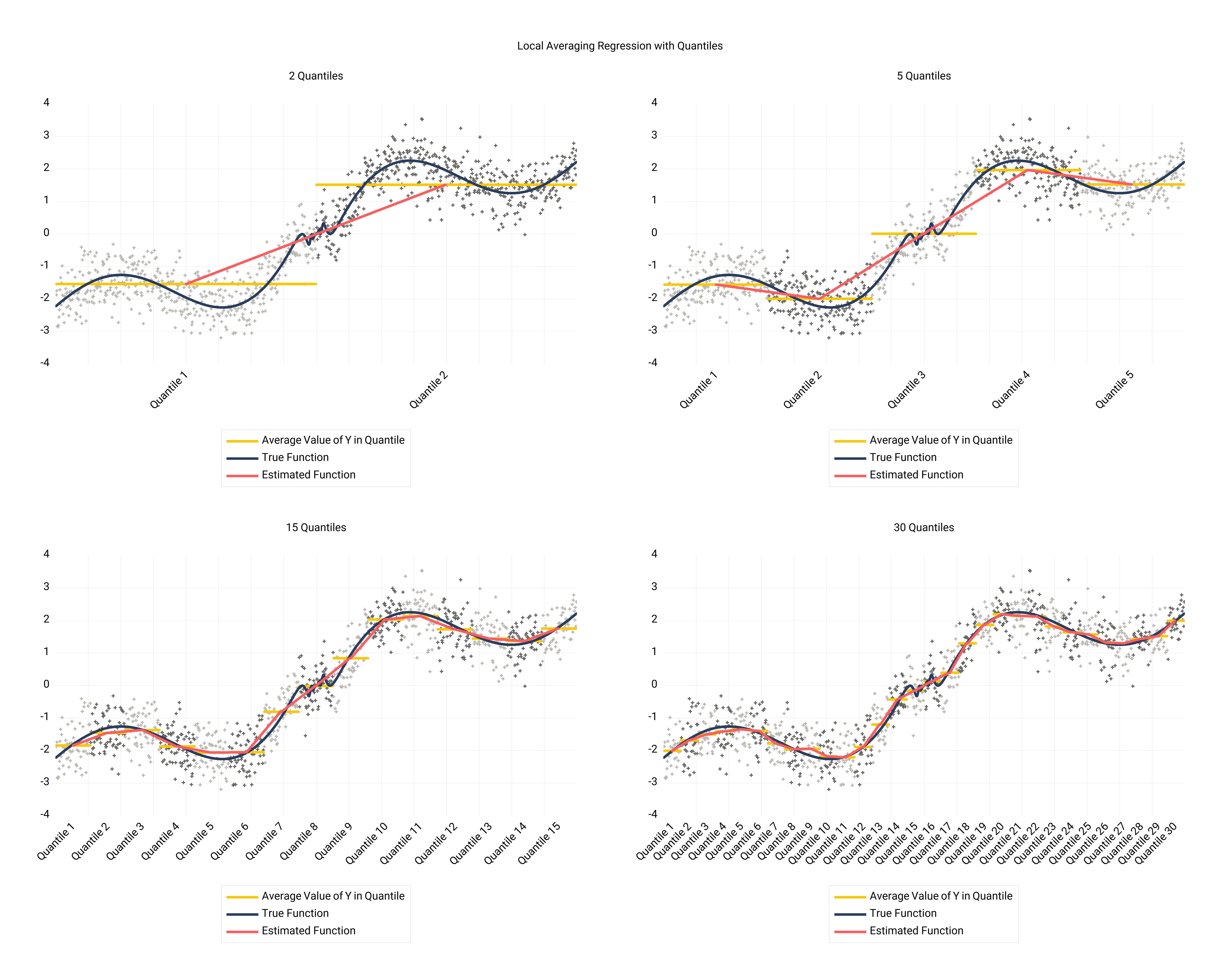
In our previous blog entry, we discussed the sign restricted VAR (SRVAR) add-in for EViews. Here, we will discuss imposing a further zero restrictions on the impact period of the impulse response function (IRF) using the ARW and SRVAR add-ins in tandem.

Table of Contents

  1. Introduction
  2. Orthogonal Reduced-Form Parameterization
  3. ARW Algorithms
  4. ARW EViews Add-in
  5. Conclusion
  6. References

Introduction

Note that it is certainly possible to impose both sign and exclusion restrictions. For example, Mountford and Uhlig (2009) are motivated by the idea that fiscal policy shocks are identified as orthogonal to both monetary policy and business cycle shocks, and use a penalty function approach (PFA) to impose zero restrictions. (For details on the PFA, please see our SRVAR blog entry.) They also considered anticipated government revenue shocks in which government revenue is restricted to rise one year following some impulse. Furthermore, Beaudry, Nam, and Wang (2011) estimate a structural VAR model including total factor productivity, stock prices, real consumption, real federal funds rate and hours worked. They use the PFA to show that a positive optimism shock causes an increase in both consumption and hours worked. Recently, Arias, Rubio-Ramirez, and Waggoner (2018), henceforth ARW, developed algorithms to independently draw from a family of conjugate posterior distributions over the structural parameterization when sign and zero restrictions are used to identify SRVARs. They showed the dangers of using the PFA when implementing sign and zero restrictions together to identify structural VARs (SVARs).

Orthogonal Reduced-Form Parameterization

ARW focus on two SVAR parameterizations. In addition to the classical structural parameterization, they show that SVARs can also be written as a product of a reduced-form parameters and a set of orthogonal matrices. This is called the orthogonal reduced-form parameterization, henceforth, ORF. The algorithms ARW propose draw from a conjugate posterior distribution over the ORF and then transform said draws into a structural parameterization. In particular, they use the normal-inverse-Wishart distribution as the prior conjugate distribution, and develop a change of variable theory that characterizes the induced family of densities over the structural parameterization. This theory shows that a uniform-normal-inverse-Wishart density over the ORF parameterization induces a normal-generalized-normal density over the structural parameterization.

To motivate their contribution, ARW first show that existing algorithms for SVARs identified only by sign restrictions, conditional on a sign restriction using the change of variable theory, operate on independent draws from the normal-generalized-normal distribution over the structural parameterization. These algorithms independently draw from the uniform-normal-inverse-Wishart distribution over the ORF parameterization and only accept draws that impose a sign restriction.

Next, ARW generalize these algorithms to also consider zero restrictions. The key to this generalization is that, conditional on the reduced-form parameters, the class of zero restrictions on the structural parameters maps to linear restrictions on the orthogonal matrices. The resulting approach generalization independently draws from normal-inverse-Wishart over the reduced-form parameters and from the set of orthogonal matrices such that the zero restrictions hold. In this regard, conditional on the zero restrictions, they show that this generalization does not induce a distribution over the structural parameterization from the family of normal-generalized-normal distributions. Furthermore, they derive the induced distribution and write an importance sampler that, conditional on the sign and zero restrictions, independently draws from normal-generalized-normal distributions over the structural parameterization.

To formalize these ideas, consider the SVAR with the general form: \begin{align} Y_t^{\prime} A_{0} = \sum_{i=1}^{p} Y_{t-i}^{\prime}A_{i} + c + \epsilon_t^{\prime}, \quad t=1, \ldots, T \label{eq1} \end{align} where $ Y_t $ is an $ n\times 1 $ vector of endogenous variables, $ A_i $ are parameter matrices of size of $ n\times n $ with $ A_{0} $ invertible, $ c $ is a $ 1\times n $ vector of parameters, $ \epsilon_t $ is an $ n\times 1 $ vector of exogenous structural shocks, $ p $ is the lag length, and $ T $ is the sample size.

We can also summarize equation \eqref{eq1} as follows: \begin{align} Y_{t}^{\prime}A_{0} = X_{t}^{\prime}A_{+} + \epsilon_{t}^{\prime} \label{eq2} \end{align} where $ A_{+}^{\prime} = \left[A_{1}^{\prime}, \ldots, A_{p}^{\prime}, c^{\prime}\right]$ and $ X_{t}^{\prime} = \left[Y_{t-1}^{\prime}, \ldots, Y_{t-p}^{\prime}, 1\right] $.

The reduced form can now be written as: \begin{align} Y_{t}^{\prime} = X_{t}^{\prime}B + u_{t}^{\prime} \label{eq3} \end{align} where $ B = A_{+}A_{0}^{-1}, u_{t}^{\prime} = \epsilon_{t}^{\prime}A_{0}^{-1} $, and $ E(u_{t}u_{t}^{\prime}) = \Sigma = \left(A_{0}A_{0}^{\prime}\right)^{-1} $. Naturally, $ B $ and $ \Sigma $ are the reduced form parameters.

We can further write equation \eqref{eq3} as the orthogonal reduced-form parameterization \begin{align} Y_{t}^{\prime} = X_{t}^{\prime}B + \epsilon_{t}^{\prime}Q^{\prime}h(\Sigma) \label{eq4} \end{align} where the $ n\times n $ matrix $ h(\Sigma) $ is the Cholesky decomposition of covariance matrix $ \Sigma $.

Given equations \eqref{eq2} and \eqref{eq4}, in addition to the Cholesky decomposition $ h $, we can define a mapping between $ \left(A_{0}, A_{+}\right) $ and $ (B, \Sigma, Q) $ by: \begin{align} f_{h}\left(A_{0}, A_{+}\right) = \left(A_{+}A_{0}^{-1}, \left(A_{0}A_{0}^{\prime}\right)^{-1}, h\left(\left(A_{0}A_{0}^{\prime}\right)^{-1}\right)A_{0}\right) \label{eq5} \end{align} where the first element of the triad on the right corresponds to $ B $, the second to $ \Sigma $, and the third to $ Q $.

Note further that the function $ f_{h} $ is invertible with inverse defined by: \begin{align} f_{h}^{-1} (B,\Sigma, Q) = \left(h(\Sigma)^{-1}Q, Bh(\Sigma)^{-1}Q\right) \label{eq6} \end{align} where the first term on the right corresponds to $ A_{0} $ and the second to $ A_{+} $.

Thus, the ORF parameterization makes clear how the structural parameters depend on the reduced form parameters and orthogonal matrices.

ARW Algorithms

Although ARW propose three different algorithms, the most important is in fact the third. The latter draws from a distribution over the ORF parameterization conditional on the sign and zero restriction and then transforms the draws into the structural parameterization. Since Algorithm 3 also depends on Algorithm 2, we present the latter here and recommend readers to refer to the supplementary materials of ARW (2018) if they require further details.

Algorithm 2

Let $ Z_j $ define the zero restriction matrix on the $ j^{\text{th}} $ structural shock, and let $ z_{j} $ denote the number of zero restrictions associated with the $ j^{\text{th}} $ structural shock. Then:
  1. Draw $ (B, \Sigma) $ independently from Normal-inverse-Wishart distribution.
  2. For $ j \in \{1, \ldots, n\} $ draw $ X_{j} \in \mathbf{R}^{n+1-j-Z_{j}} $ independently from a standard normal distribution and set $ W_{j} = X_{j} / ||X_{j}||$.
  3. Define $ Q = [q_{1}, \ldots q_{n}] $ recursively as $ q_{j} = K_{j}W_{j} $ for any matrix $ K_{j} $ whose columns form an orthonormal basis for the null space of the $ (j-1+z_{j})\times n $ matrix \begin{align} M_{j} = \left[q_{1}, \ldots, q_{j-1},\left(Z_{j}F\left(f_{h}^{-1}(B, \Sigma, I_{n})\right)\right)\right] \end{align}
  4. Set $ (A_{0},A_{+}) = f_{h}^{-1}(B,\Sigma,Q) $.

Algorithm 3

Let $ \mathcal{Z} $ denote the set of all structural parameters that satisfy the zero restrictions, and define $ v_{(g^{\circ}f_{h})|\mathcal{Z}} $ as te volume element. Then:
  1. Use Algorithm 2 to independently draw $ (A_{0}, A_{+}) $.
  2. If $ (A_{0}, A_{+}) $ satisfies the sign restrictions, set its importance weight to $$ \frac{|\det(A_{0})|^{-(2n+m+1)}}{v_{(g^{\circ}f_{h})|\mathcal{Z}}(A_{0}A_{+})} $$ otherwise, set its importance weight to zero.
  3. Return to Step 1 until the required number of draws has been obtained.
  4. Re-sample with replacement using the importance weights.

ARW EViews Add-in

Now we turn to the implementation of the ARW add-in. First, we need to download and install the add-in from the EViews website. The latter can be found at https://www.eviews.com/Addins/arw.aipz. We can also do this from inside EViews itself. In particular, after opening EViews, click on Add-ins from the main menu, and click on Download Add-ins.... From here, locate the ARW add-in and click on Install.


Figure 1: Add-in installation

After installing, we open the data file named as data.WF1 which can be found in the installation folder, typically located in [Windows User Folder]/Documents/EViews Addins/ARW.


Figure 2: ARW (2018) Data

We now replicate Figures 1 and Table 3 from ARW. We can of course do this in EViews as follows.

  1. Click on the Add-ins menu item in the main EViews menu, and click on Sign restricted VAR.
  2. Under Endogenous variables enter tfp stock cons ffr hour.
  3. Check the Include constant option.
  4. Under Number of lags, enter 4.
  5. In the Sign restriction vector textbox enter +2.
  6. Under Sign restriction method check Penalty.
  7. In the Number of horizons enter 40
  8. Under Zero restriction textbox enter tfp.
  9. Check the variance decomposition box.
  10. Hit OK.


Figure 3: SRVAR Add-in (PFA)

The steps above produce the following output (Panel A of Figure 1 of ARW):


Figure 4: PFA Output

Next, we invoke the ARW add-in and proceed with the ARW Algorithm 3.

  1. Click on the Add-ins menu item in the main EViews menu, and click on Sign and zero restricted VAR.
  2. Under Endogenous variables enter tfp stock cons ffr hour.
  3. Check the Include constant option.
  4. Under Number of lags, enter 4.
  5. In the Sign restriction vector textbox enter +stock.
  6. In the Zero restrictions textbox enter tfp.
  7. UnderNumber of steps enter 40.
  8. Check the variance decomposition box.
  9. Hit OK.


Figure 5: ARW Add-in (Importance Sampler)

The steps above produce the following output (Panel B of Figure 1 of ARW):


Figure 6: Importance Sampler Output

Figures 5 and 6 above illustrates the IRFs using the PFA and importance sampler methods, respectively. In case of the former, we can see the IRFs with probability bands for adjusted TFP, stock prices, consumption, real interest rate,and hours worked under the PFA. Examining the confidence bands around IRFs allows us to conclude that optimism shocks boost consumption and hours worked, as the corresponding IRFs do not contain a zero for at least 20 quarters.

Alternatively, the IRFs of the same variables obtained using the importance sampler yield a different result. For consumption and hours worked, the confidence bands are wider and contain zero. Furthermore, the corresponding point-wise median IRFs are closer to zero compared to those obtained using the PFA. This shows that the PFA exaggerates the effects of optimism shocks on stock prices, consumption, and hours worked, by generating much narrower confidence bands and larger point-wise median IRFs. In this regard, as pointed out by Uhlig (2005), we can see that the PFA includes additional identification restrictions when implementing sign and zero restrictions.

To further summarize the results, we present the table below which gives the specifics of the output figures above.

Penalty Function ApproachImportance Sampler
Adjusted TFP0.070.170.290.030.110.23
Stock Prices0.540.720.840.050.290.57
Consumption0.130.270.430.030.170.50
Real Interest Rate0.070.140.230.080.200.39
Hours Worked0.200.310.450.040.180.56
Table I: Forecast Error Variance Decomposition (FEVD)

Table I shows the contribution of shocks to the Forecast Error Variance Decomposition (FEVD) using the PFA and the importance sampler for the chosen horizon of 40 periods and 68 percent equal-tailed probability intervals. Under the PFA, the share of FEVD attributable to optimism shocks of consumption and hours worked is 27 and 31 percent, respectively. However, the contribution of optimism shocks to the FEVD of stock prices is 72 percent under the PFA in contrast to 29 percent using the importance sampler. It should be noted that for most variables, when using the importance sampler, optimism shocks contribute less to the FEVD, and probability intervals for the FEVD are broader as opposed to those obtained under the PFA.

Conclusion

In this blog entry we presented the ARW add-in for EViews. The add-in is based on the work of ARW (2018) and generates impulse response curves based on the importance sampler which accommodates both sign and zero restrictions in the VAR model.


References

  1. Arias J., Rubio-Ramirez J., and Waggoner D.: Inference Based on SVARs Identified with Sign and Zero Restrictions: Theory and Applications Econometrica, 86:685–720, 2018.
  2. Beaudry P., Nam D., and Wang J.: Do mood swing drive business cycle and is it rational? NBER Working Paper 17651, 2011.
  3. Mountford A. and Uhlig H.: What are the effects of fiscal policy shocks? Journal of Applied Econometrics, 24:960–992, 2009.
  4. Uhlig H.: What are the effects of monetary policy on output? Results from an agnostic identification procedure. Journal of Monetary Economics, 52(2):381–419, 2005.
Viewing all 69 articles
Browse latest View live